2020-2학기 서강대 김경환 교수님 강의 내용 및 패턴인식 교재를 바탕으로 본 글을 작성하였습니다.
9.6 Estimating and comparing classifiers (분류기 추정 및 비교)
▶ Two reasons for wanting to know the generalization rate of a classifier on a given problem.
- To see if the classifier performs well enough to be useful.
- To compare its performance with that of a competing design.
주어진 문제에 대한 분류기의 "generalization rate"을 알고자 하는 데, 적어도 두 가지 이유가 존재한다.
- 첫째, 분류기가 충분히 쓸모 있게 잘 수행하는가를 확인하는 목적
- 둘째, 비교 상대의 성능과 비교하려는 것
9.6.1 Parametric Models
- To compute the generalization rate from the assumed parametric model.
- There are three problems with the approach:
"Generalization ration"를 추정하는 방법은 "parametric model"로 가정을 하고 계산할 수 있으나, 세가지 문제점을 아래와 같이 가지고 있다.
- An error estimate is overly optimistic.
- We should suspect the validity of an assumed parametric model.
- It is very difficult to compute the error rate exactly in more general situations where the distributions are not simple.
첫째, 그러한 에러 추정은, 보통 지나치게 낙관적이다. 훈련 샘플들을 특이하거나 비전형적이게 만드는 특성들이 드러나지 않음
둘째, 항상 가정된 파라미터형 모델의 유효성을 의심해야함. 똑같은 모델에 기반한 성능 평가를 그 평가가 불리하지 않는 한 신뢰할 수 없음
셋째, 분포가 단순하지 않은 더 일반적인 상황들에서 에러율을 정확하게 계산하는 것은 확률 구조가 완전히 알려져 있다고 해도 매우 어렵다.
9.6.2 Cross-Validation
- A validation set is used to estimate the generalization error
- The set of labeled training samples
- The traditional training set for adjusting model parameters
- The validation set for estimating the generalization error
- It is essential that the validation set not include points used for training the parameters in the classifier.
★ 주의점 : validation 및 test 진행 시, 분류기의 parameter들은 반드시 훈련시키지 말아야 한다. 그렇지 않으면, "훈련 집합에 대한 시험"이라고 알려진 방법론적 오류를 범하게 된다.

▶ Cross-Validation
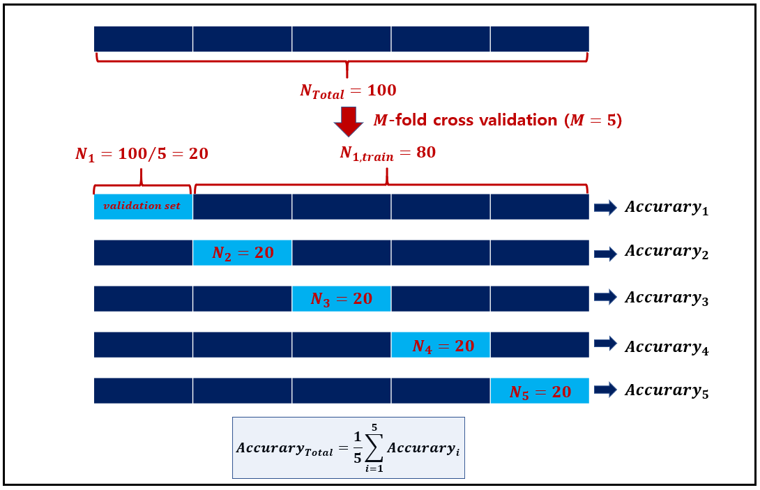
- M-fold cross-validation : a simple generalization of the method
위 방법에 대한 간단한 "generalization"가 "M-fold cross validation"이며, 절차는 다음과 같다.
- The training set is randomly divided into $m$ disjoint sets of equal size $n/m$.
- The classifier is training $m$ times, each time with a different set held out as a validation set.
- The estimated performance is the mean of these $m$ errors
- Heuristics for choosing the portion of $D$ to be used as a validation set.
validation 기법은 heuristics 기법이며, 모든 경우에서 개선된 분류기들을 제공할 필요는 없음(사실상 불가능), 그럼에도 불구하고 validation 기법은 간단하며, 많은 일반화 성능을 향상시키는 것으로 확인되고 있음, validation 집합으로 사용될 $D$의 일정 비율 $0 \lt \gamma \lt 1$를 선정하기 위한 몇 가지 heuristics들이 있음.
default로 $\gamma=0.1$로 설정하며, 일반적으로 0.5보다 작은 값 설정함
- Cross-validation is an empirical approach that tests the classifier experimentally.
cross-validation은 그 바탕은 분류기를 실험적으로 시험하는 경험적 방식이다.
- If the true but unknown error rate of the classifier is $p$ and if $k$ of the $n’$ independent, randomly drawn test samples are misclassified. Then MLE for $p$
$$\hat{p} = \frac{k}{n'} \tag{1}\label{1}$$
- $n'$ : test data sets 갯수 (train과 독립적으로 추출됨)
- $k$ : test set에서의 오분류된 갯수
- $\hat{p}$ : 오분류된 test data sets의 비율 ($p$에 대한 추정)
- The $95%$ confidence intervals for a given estimated error prob.
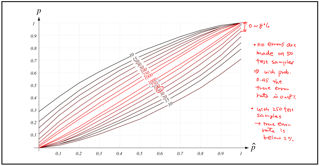
이항 분포의 parameter의 $p$에 대한 이 추정의 특성들은 잘 알려져 있음, 특히 위 그림은 95%신뢰 구간들을 $\hat{p}$와 $n'$과의 함수로 보여준다. 주어진 $\hat{p}$의 값에 대해 $p$의 참 값이 test sample n'에 의해 표시된 아래쪽 그림과 위쪽 곡선들 사이의 구간에 놓이는 확률은 0.9다.
- $n$이 증가할수록 error prob가 감소하는 것을 알 수 있음 ($n=50 \rightarrow 0~8%, n = 250 \rightarrow 0~2%$)
위 곡선은 $n'$이 작은 경우, 최대-우도 추정을 해석할 때 주의가 필요함을 보여준다. (즉, 데이터 수가 적은 경우, True와의 Error가 더 넓어지는 것을 확인할 수 있다는 이유에서)
9.6.3 Jackknife and Bootstrap Estimation of Classification Accuracy
- A method for comparing classifiers closely related to cross-validation is to use the jackknife or bootstrap estimation procedures
cross-validation과 밀접하게 관련된 분류기들을 비교하기 위한 방법은 Jackknife 또는 Bootstrap 추정을 이용하는 것이다.
▶ For the jackknife method
- By training the classifier $n$ separate times, each time using the training set $D$ from which a different single training point has been deleted.
- Each resulting classifier is tested on the single deleted point, and the jackknife estimate of the accuracy is then simply the mean of these leave-one-out accuracies.
분류에 대한 Jackknife 기법의 응용은 간단하다. 주어진 알고리즘의 정확도를 분류기를 $n$번 훈련시켜서 추정하되, 훈련 집합 $D$에서 매번 다른 point 한 개를 빼고 사용하는 것이다. (즉 $M$-fold cross validation에서 $M$를 $D$의 전체 갯수 $n$으로 설정, 즉 $M=n$) 각결과 분류기는 제외된 한 point 에 대해 시험되며, 정확도의 jackknife 추정은 단순히 이들 한 샘플 제외(leave-one-out) 정확도들의 평균이다. (단, 계산 복잡도는 매우 높을 수도 있음)
- A particular benefit of the jackknife is that it can provide measures of confidence or statistical significance in the comparison between two classifier designs
특히 Jackknife 기법은 $n$개 분류기의 각각이 시험될 분류기와 아주 비슷하기 때문에 일반적으로 훌륭한 추정들을 제공한다. Jackknife 방식의 특별한 이점은 두 분류기 설계 간의 비교에서 신뢰 또는 통계적 중요성의 척도를 제공할 수 있다. (예시를 통해 알아보자)
- $C_1$ has $80%$ accuracy
- $C_2$ has $85%$ accuracy
Is $C_2$ reallay better $C_1$ ?
이에 답하기 위해, 분류 정확도들의 variance의 Jackknife 추정을 계산하고, 전통적 가설 검증을 사용해서 $C_1$의 왼견상 우월성이 통계적으로 의미가 있는지를 알아본다. (아래 그림 참고)

즉, $C_2$의 정확도가 $C_1$보다 높아보이지만, Jackkife 추정을 이용해 분류기의 variance 관점에서는 $C_2$보다 $C_1$이 우월해 보임을 보여주고 있음
▶ For the bootstrap method
- To training B classifiers, each with a different bootstrap data set, and test on other bootstrap data set.
- The classifier accuracy is simply the mean of these bootstrap accuracies.
부트스트랩 방법을 분류기의 정확도를 추정하는 문제로 일반화시는 몇가지 방법이 있다. 가장 간단한 방식 중 하나는 $B$개 분류기를 각각 서로 다른 부트스트랩 데이터 집합으로 훈련시키고, 다른 부트스트랩 데이터 집합들에 대해 시험하는 것이다.
분류기 정확도의 부트스트랩 추정은 단순이 이 부트스트랩 정확도들의 평균이고, 실제로, 분류기 정확도의 부트스트랩 추정의 높은 계산 복잡도는 때때로 추정 가능한 개선들과 연관이 있음
9.6.4 Maximum-Likelihood Model Comparison
▶ For the bootstrap method
- The goal is to choose the model that best explains the training data.
$$
P\left(h_{i} \mid D\right)=\frac{P\left(D \mid h_{i}\right) P\left(h_{i}\right)}{p(D)} \propto P\left(D \mid h_{i}\right) P\left(h_{i}\right) \tag{2}\label{2}
$$
- The data-dependent term, $P(D|h_i)$, is the evidence for $h_1$.
- $P(h_i)$ is subjective prior over the space of hypotheses and often neglected in the computation.
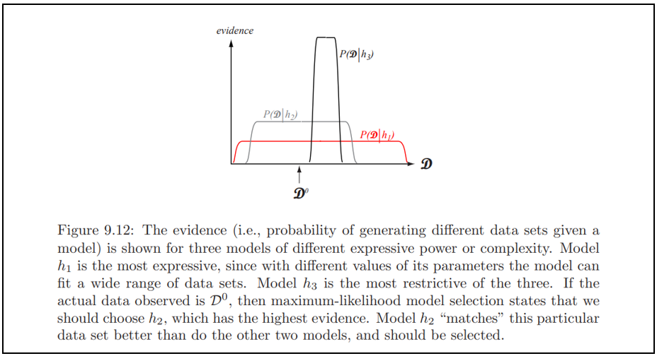
[그림 5]는 서로 다른 모델들에 대해 evidence를 보여주고 있음, 모델 $h_1$은 parameter들의 서로 다른 값에 의해 이 모델이 넓은 범위의 데이터 집합들을 맞출 수 있기 때문에 가장 표현적이다. 반면에 $h_3$는 셋중 가장 제약적이다. 관찰된 실제 데이터가 $D^0$라면, 최대-우도 모델 선택은 우리가 가장 높은 Evidence를 갖는 $h_2$를 선정해야 한다. 모델 $h_2$는 이 특정 데이터 집합 $D^0$을 다룬 두 모델보다 더 잘 "맞추기" 때문에, $D^0$라는 데이터 내에서는 선택되어야 함
추가적으로 두 번째 계수인 $P(h_i)$는 가설들의 공간에 대한 우리의 주관적 사전 확률이다. (데이터를 알기 전에 서로 다른 모델에 대한 우리의 믿음/신뢰를 의미함). 흔히, 계산에서 무시되는 경우가 있음.
9.6.5 Bayes Model Comparison (교과서 읽기, skip)
▶ Bayesian model comparison uses the full information over priors when computing posterior probabilities.
사후 확률들을 계산할 때 사전 확률들에 대한 전체 정보를 사용함
9.6.6 The Problem-average Error Rate
▶ The examples thus far suggest that the problem with having only a small number of samples is that the resulting classifier will not perform well on new data.
▶ We expect the error rate to be a function of the number n of training samples.
▶ Analytical investigation
- Estimate the unknown parameters from samples.
- Use these estimates to determine the classifier.
- Calculate the error rate for the resulting classifier.
이제까지 제공한 예제들은 적은 수의 샘플만을 가질 때의 문제는 그 결과 분류기가 새로운 데이터에 대해 제대로 성능을 내지 못하는 (generalization되지 않음) 것을 암시한다. 따라서 error ratio가 훈련 샘플 $n$의 함수라고 예상할 수 있다. (보통 $n$이 무한대로 감에 따라 어떤 최솟값까지 감소할 것). 이를 분석적으로 탐색하기 위해 위 단계를 수행해야 함
This analysis is very complicated. (복잡함)
▶ By using histogram approximations to the unknown probability densities and averaging appropriately, it is possible to draw some illuminating conclusions.
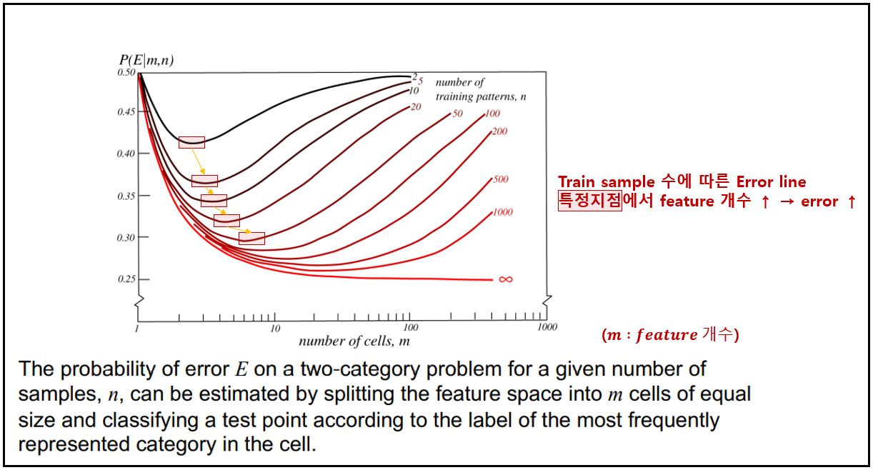
주어진 샘플 수에 대한 2-category classification 문제에서 error $E$의 확률은 특징 공간을 같은 크기의 $m$개의 cell로 나누고 test point을 그 cell에서 가장 빈벊게 대표되는 부류의 레이블에 따라 분류해서 추정될 수 있음, 위 그래프들은 $m$과 $n$이 표시된 많은 random 문제의 평균 에러를 보여주고 있음
9.6.7 Predicting Final Performance from Learning Curves
▶ Training on very large data sets can be computationally intensive.
▶ We seek a method to compare classifiers without the need of training all of them fully on the complete data set.
매우 큰 데이터 집합들에 대해 훈련시키는 것은 계산적으로 부담스러울 수 있으며, 강력한 PC에서도 오래 걸릴 수 있으므로, 현실적으로 전체 데이터를 모두 학습시킬 필요 없이, 분류기들을 비교하는 방법이 필요하다. 만일 가장 유력한 모델을 빠르고 효율적으로 결정할 수 있다면, 우리가 해야 하는 모든 것은 이 모델을 완전하게 훈련시키는 것이다.
- One method is to use a classifier’s performance on a relatively small training set to predict its performance on the ultimate large training set.
- Such performance is revealed in a type of learning curve.
한 방법은 최종적인 큰 훈련 집합에 대한 분류기의 성능을 예측하기 위해 비교적 작은 훈련 집합에 대한 그것의 성능을 이용하는 것이고, 그러한 성능은 훈련 집합의 크기에 대한 시험 에러를 보여주는 어떤 유형의 학습 곡선에서 드러난다.
9.6.8 The Capacity of a Separating Plane (skip)
▶ All dichotomies of $d+1$ or fewer points are linear.
▶ The capacity of a hyperplane: $n=2(d+1)$
...
9.6 Estimating and comparing classifiers (분류기 추정 및 비교)
▶ Mixture-of-expert models, ensemble classifiers, modular classifiers, or occasionally pooled classifiers.
- Useful if each of the component classifiers is highly trained in a different region of the feature space.
- Mixture distribution

- The mixture-of-experts


댓글