2020-2학기 서강대 김경환 교수님 강의 내용 및 패턴인식 교재를 바탕으로 본 글을 작성하였습니다.
9.3 Bias and variance
▶ Given that there is no general best classifier unless the probability over the class of problems is restricted, practitioners must be prepared to explore a number of methods or models when solving any given classification problem.
문제들의 클래스에 대한 확률이 제한되지 않는 한 범용의 최선의 분류기는 없다고 주어지면, 우리는 주어진 분류 문제를 풀 때 여러 방법 또는 모델을 탐구할 준비가 되어 있어야 한다. 아래에는 분류 문제에 대한 학습 알고리즘의 "match" 및 "alignment"를 측정하는 두 가지 방법을 정의할 것이다. (단, control이 불가능한 noise에 대해서는 잠시 접어두기로 하자)
Bias
- measures the accuracy or quality of the match. (match의 정확도)
- High bias implies a poor match.
Variance
- measures the precision or specificity of the match. (match의 정밀도)
- High variance implies a weak match.

분류기의 bias와 variance를 조정할 수 있으나, 조정할 때의 주의점은 bias와 variance의 관계는 서로 trade-off 관계가 있음을 유념하자.
9.3.1 Bias and Variance for Regression
bias, variance의 개념은 regression / curve fitting 문맥에서 가장 쉽게 이해할 수 있음
$$
\begin{aligned}
&E_{D}\left[(g(\mathbf{x} ; D)-F(\mathbf{x}))^{2}\right]=\underbrace{\left(E_{D}[g(\mathbf{x} ; D)-F(\mathbf{x})]\right)^{2}}_{\text {bias }^{2}}+\underbrace{E_{D}\left[\left(g(\mathbf{x} ; D)-E_{D}[g(\mathbf{x} ; D)]\right)^{2}\right]}_{\text {variance }}\\
&\begin{array}{l}
\end{array}
\end{aligned} \tag{1}\label{1}
$$
- $g(\mathbf{x} ; D)$ : function estimated ($D$로부터 추정된 함수)
- $F(\mathbf{x})$ : true but unknown (미지의 함수 : True 함수)
▶ low bias
- accurate estimate of $F$ from $D$ (평균적으로 $D$로부터 $F$를 정확하게 추정)
▶ low variance
- estimate of $F$ does not change much as the training set varies. (train set이 바뀌어도 많이 변하지 않음을 의미)
▶ Bias-Variance Dilemma (trade-off)
- Procedures with increased flexibility to adapt to the training data (e.g., have more free parameters) tend to have lower bias but higher variance.
훈련 데이터에 적응하는 증가된 유연성을 갖는(예를 들면, 더 많은 파라미터를 갖는) 프로시저들은 더 낮은 bias와 더 높은 variance를 갖는 경향이 있음

예를 들어, True Function $F(\mathbf{x}$가 아래 [그림 1]과 같이 noise가 있는 한 변수의 3차 다항식(검정 실선)이라고 하자. 샘플링된 train data 집합 $D_{1}, D_{2}, D_{3}, ...$에 기초해서 이 함수를 추정하기를 원할때, bias, variance 관점에서 보자.

- $a$ : parameter들이 모든 train data ($D_{1}, D_{2}, ...$)와 독립적으로 fixed 이므로 variance는 0이지만, bias가 매우 큼 (불충분한 모델)
- $b$ : parameter들이 모든 train data ($D_{1}, D_{2}, ...$)와 독립적으로 fixed 이므로 variance는 0이지만, $a$에 비해 bias가 상대적으로 작음 (다소 나은 모델)
- $c$ : 3차 항을 가지는 $g(\mathbf{x})$의 parameter들은 train data($D_{1}, D_{2}, ...$)마다 다르게 설정될 것이다. 따라서 variance는 커지며, 반대로 bias는 낮은 bias를 볼 수 있음
- $d$ : 1차 항을 가지는 $g(\mathbf{x})$의 parameter들은 train data($D_{1}, D_{2}, ...$)마다 다르게 설정될 것이다. 따라서 variance는 존재하지만, 상대적으로 차수가 높은 $c$보다 variance는 적을 것이다. 하지만 bias는 $c$보다 다소 높음
지금까지 regression problem에서의 bias와 variance의 정의 및 둘 사이의 trade-off 관계를 살펴보았다. 다음 ch9.4에서는 classification(분류)에서의 bias 및 variance의 관계를 알아보도록 하겠다.
9.3.2 Bias and Variance for Classification
▶ Much as we saw in the bias-variance dilemma for regression, classification procedures with increased flexibility to adapt to the training data (e.g., have more free parameters) tend to have lower bias but higher variance.
regression의 경우. bias-variance decomposition(분해)와 trade-off 관계를 이해하기 수월했었다. 이번 ch9.4는 regression이 아닌 classifiaction의 경우에서의 bias-variance의 관계를 살펴보고자 한다.
▶ An illustration of boundary bias and variance in classifiers.
- Two-class problem in which samples are drawn from two-dimensional Gaussian distributions.
분류에서의 bias-variance trade-off를 2-차원 가우시안 분포를 이용해서 예를 들어보겠다.
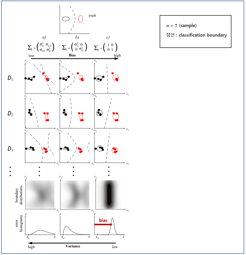
▶ Column a-most general Gaussian classifiers
- Left column – very low bias, right – high bias
▶ Each row represent a different training set, and the resulting classifiers.
- Low-bias case: high variance
- High-bias case: low variance
▶ The density plots show how the location of the decision boundary varies across many different training set
- Leftmost : a very broad distribution (high variance)
- Rightmost : peaked distribution (low variance)
▶ For a given bias, the variance will decreases as n is increased.
bias가 주어진 경우, $n$이 증가할 수록 variance는 낮아질 것이다.
[그림 3]에 대해 해석하면 다음과 같이 정리할 수 있다.
- $a$ : MLE에 의해 훈련된 완전히 일반적인 공분산 행렬들을 갖는 가우시안 분포로 모델 : 학습된 경계들을 데이터 집합 간에 현저히 다름 ; 이 학습 알고리즘은 높은 variance을 가짐
- $b$ : MLE에 의해 훈련된 대각선형 공분산 행렬들을 가지는 가우시안 분포로 모델 : 학습된 경계들은 $D$에 따라 달라지기는 하지만 $a$보다 덜한 variance을 가짐
- $c$ : MLE에 의해 훈련된 단위 공분산 행렬들을 가지는 가우시안 분포로 모델(선형 모델) : $D$에 대해 판정 경계가 거의 동일함에 주목하자. 가장 낮은 variance를 가짐.
▶ To achieve the desired low generalization error it is more important to have low variance than to have low bias.
- The only way to get the ideal of zero bias and zero variance is to know the true model ahead of time – no learning was needed.
- Bias and variance can be lowered with large training size $n$ and accurate prior knowledge.
- As $n$ grows, more parameters must be added to the model, g, so the data can be fit (reducing bias).
<참고>
classification에서는 원하는 낮은 일반화 에러를 달성하려면 낮은 bias를 갖는것보다 낮은 variance를 갖는게 더 중요함. (이에 대해서는 책을 참고하면 실마리를 얻을 수 있음)
▶ For best classification based on a finite training set, it is desirable to match the form of the model to that of the (unknown) true distributions;
- This usually requires prior knowledge.


댓글