2020-2학기 서강대 김경환 교수님 강의 내용 및 패턴인식 교재를 바탕으로 본 글을 작성하였습니다.
5.2 Linear Discriminant Functions and Decision Surfaces
$\mathbf{x}$의 요소들의 선형 결합인 판별 함수는 다음과 같이 쓸 수 있다.
$$g(\mathbf{x})=\mathbf{w}^T \mathbf{x} + \omega_0 \tag{1}\label{1}$$
- $\mathbf{x}$ : weight vector
- $\omega$ : bias (or threshold weight)
Ch2에서 보았듯이 일반적인 $c$개의 class 분류라면 $c$개의 판별 함수가 있을 것이다.
▶ The Two-Category Case (cont.)
식 (1) 형태의 판별 함수에 대해, Two-category case라면 다음의 decision rule을 구현하면 된다. (사실 한 개의 discriminant function만 존재해도 분리 가능함)
$g(\mathbf{x}) \gt 0$ 이면, $\omega_1$으로 판정하고, $g(\mathbf{x}) \lt 0$이면 $\omega_2$로 판정한다. 즉 $\mathbf{x}$는 내적(inner product) $\mathbf{w}^T \mathbf{x}$가 $-\omega_1$를 넘으면 $\omega_1$으로 할당, 그렇지 않으면 $\omega_2$로 할당된다. 만일 $g(\mathbf{x})$가 0이라면 $\mathbf{x}$를 보통 아무 class로 할당될 수 있으나, 이 장에서는 그 할당을 정의되지 않은 채로 두자. 아래 그림 5.1은 일반적인 선형 분류기를 보여주고 있다.
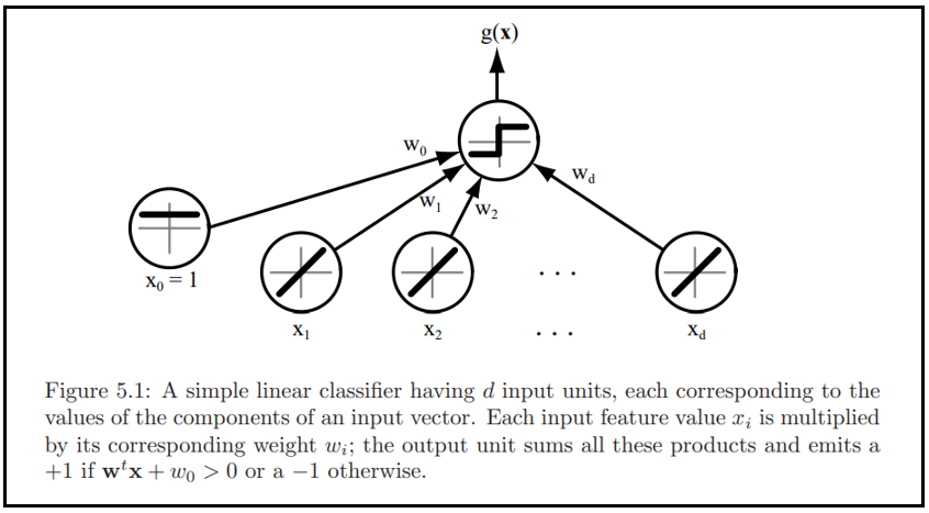
- $g(\mathbf{x}) = 0$ defines the decision surfaces (hyperplane)
만일, $\mathbf{x}_1$과 $\mathbf{x}_2$가 모두 decision surface에 있다면
$$\mathbf{w}^T \mathbf{x}_1 + \omega_0 = \mathbf{w}^T \mathbf{x}_2 + \omega_0 \tag{2}\label{2}$$
또는
$$\mathbf{w}^T (\mathbf{x}_1 - \mathbf{x}_2) = 0 \tag{3}\label{3}$$
이며, 이는 $\mathbf{w}$가 hyperplane에 놓인 어떠한 벡터에 대해서도 수직(orthogonal)임을 나타낸다.
일반적으로 hyperplane(H)는 특징 공간을 두 개의 half-space로 나누게 되며, $\omega_1$을 위한 판정 영역 $R_1$과 $\omega_2$를 위한 판정 영역 $R_2$로 구분된다.
- $g(\mathbf{x})$ gives an algebraic measure of the distance from $\mathbf{x}$ to the hyperplane
판별 함수 $g(\mathbf{x})$는 $\mathbf{x}$로부터 초평면까지의 대수학적 거리 척도를 제공한다.
$$
\mathbf{x}=\mathbf{x}_{p}+r \frac{\mathbf{w}}{\|\mathbf{w}\|} \tag{4}\label{4}
$$

$\mathbf{x}$가 "+" 쪽에 있으면 양, $\mathbf{x}$가 "-"쪽에 있으면 음이다. 또한, $g(\mathbf{x}_p) = 0$이므로,
$$g(\mathbf{x}) = \mathbf{w}^T \mathbf{x} + \omega_0 = r ||\mathbf{w}|| \tag{5}\label{5}$$
또는
$$r = \frac{g(\mathbf{x})}{||\mathbf{w}||} \tag{6}\label{6}$$
이다. 식 (5), (6)에 대한 전개 과정은 아래를 참고하자.
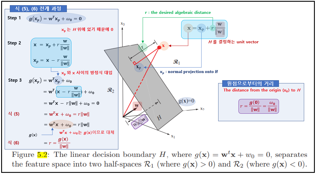
- The distance from the orgin to $H$ : $\frac{\omega_0}{||\mathbf{w}||}$
만일 $\omega_0 \gt 0$이면 원점은 $H$의 양 족에 있으며, $\omega_0 \lt 0$이면 음 쪽에 있다. $\omega_0 = 0$이면 $g(\mathbf{x})$는 homogeneous 형태 $\mathbf{w}^T \mathbf{x}$를 가지며 초평면은 원점을 지난다. 위 그림 5.2가 결과들을 기하학적으로 보여준다.
Summary
- A linear discriminant function divides the feature space bya hyperplane decision surface.
- The orientation of $H$ is determined by the normal vector $\mathbf{w}$. (표면 방향)
- The location of the $H$ is determined by the bias $\omega_0$. (표면의 위치)
- 판별 함수 $g(\mathbf{x})$는 $\mathbf{x}$에서 초평면까지의 부호 있는 거리에 비례하며, $\mathbf{x}$가 양 쪽에 있을 때는 $g(\mathbf{x}) \gt 0$, $\mathbf{x}$가 음쪽에 있을 때는 $g(\mathbf{x}) \lt 0$이다.
▶ The Multi-Category Case (cont.)
선형 판별 함수를 사용하는데 multi-class classifier를 고안하는 다양한 방법이 있다.
- $c$ two-class problems ($c$개의 2-클래스 문제)
예를 들면 위와 같이 $c$개의 클래스 문제로 축소시킬 수 있다. 여기서는 $i$번째 문제는 $\omega_i$에 할당된 점들을 그렇지 않은 점들로부터 분리(two-class라고 하는 이유)하는 선형 판별 함수에 의해 풀리며, 아래 그림과 같다.

- $c(c-1)/2$ linear discriminants (one for every pair of classes)
더 낭비적인 방법인 클래스 쌍에 대해 하나씩, 즉 $c(c-1)/2$개의 선형 판별식을 사용하는 것이다.

이런 모호한 경계선에 대한 문제점을 해결하기 위해 Ch2에서 택한 아래 방정식을 적용하고자 한다. $c$개의 선형 판별 함수를 다음과 같이 정의하고,
$$
g_{i}(\mathbf{x})=\mathbf{w}^{t} \mathbf{x}_{i}+w_{i 0} \quad i=1, \ldots, c \tag{7}\label{7}
$$
모든 $j \neq i$에 대해 $g_i(\mathbf{x}) \gt g_j(\mathbf{x})$이면 $\mathbf{x}$를 $\omega_i$에 할당한다; 동률인 경우, 분류는 정의되지 않은 상태로 남긴다. 이러한 분류기를 linear machine(선형 기계)라고 부르는데, 특징 공간을 $c$개의 판정 영역으로 나누며, 이때 $g_i(\mathbf{x})$는 $\mathbf{x}$가 영역 $R_1$에 있으면 최대 판별식이다. 만일 $R_i$와 $R_j$가 붙어 있으면, 둘 사이의 경계는 다음에 의해 정의되는 초평면 $H_{ij}$의 일부이다.
$$g_i(\mathbf{x}) = g_j(\mathbf{x}) \tag{8}\label{8}$$
또는
$$
\left(\mathbf{w}_{i}-\mathbf{w}_{j}\right)^{T} \mathbf{x}+\left(w_{i 0}-w_{j 0}\right)=0 \tag{9}\label{9}
$$
바로 당연한 결과로서 $\mathbf{w}_i -\mathbf{w}_j$는 $H_{ij}$에 수직이며, $\mathbf{x}$에서 $H_{ij}$까지의 부호 있는 거리는 아래와 같이 주어진다.
$$
\frac{\left(g_{i}-g_{j}\right)}{\left\|\mathbf{w}_{i}-\mathbf{w}_{j}\right\|} \tag{10}\label{10}
$$
- It is not the weight vector themselves but thier differences that are important.
- The total number of hyperplane segments in the decision surfaces is often fewer than $c(c-1)/2$.
영역 쌍의 수는 $c(c-1)/2$이지만 모두 인접할 필요는 없으며 판정 평면들에 나타나는 초평면 세그먼트들의 전체 수는 흔히 그림 5.4에서 보듯이 $c(c-1)/2$보다 적다.

Reference
'Pattern Classification [수업]' 카테고리의 다른 글
| Ch7.1 Stochastic Methods - Introduction (0) | 2020.11.17 |
|---|---|
| Ch5.3 Linear Discriminant Functions - Generalized linear discriminant functions (0) | 2020.11.02 |
| Ch5.1 Linear Discriminant Functions - Introduction (0) | 2020.10.29 |
| Ch4.3 Nonparametric techniques - Parzen Windows (0) | 2020.10.12 |
| Ch4.2 Nonparametric techniques - Density Estimation (0) | 2020.10.07 |


댓글