2021-1학기 서강대 김홍석 교수님 강의 내용을 바탕으로 본 글을 작성하였습니다.
Overview
- Markov Processes
- Markov Reward Processes
- Markov Decision Processes
- Entensions to MDPs
ch2는 model based 기반 MRP, MDP에 대한 정의 및 예제를 다루고자 한다. 이후 ch3에서 MDP를 푸는 방법을 다룰 것이다.
1. Markov Processes
▶ Introduction to MDPs
- MDPs (Markov decision processes) formally describe an environment for reinforcement learning
- Where the environment is fully observable
MDPs는 강화학습에서의 environment(환경)을 수식적(공식)으로 표현할 수 있다. 여기서의 environment는 fully observable이며, 이는 다음과 같은 수식을 가진다. $P(s',a' | s, a)$
- i.e. The current state completely characterieses the processes
- Almost all RL problems can be formalised as MDPs
$S_t$(현재 상태)는 Markov Property 정의에 따라 process를 결정하며, MDPs는 순차적으로 행동을 계속 결정하는 문제를 수학적으로 표현한 것이다.
MDP를 다루기전 이해를 돕기 위해 더 작은 문제 순으로 Markov Processes → Markov Reward Processes → Markov Decision Processes(MDPs) 알아보도록 하자.
▶ Markov Property
- "The future is independent of the past given the present"
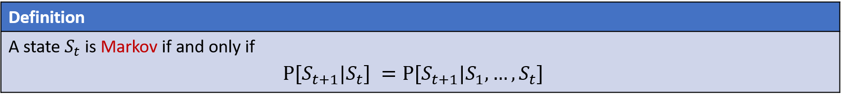
어떤 $t$ 시점에서의 상태인 $S_t$가 Markov 라고 하면, 동치는 다음과 같다. $S_t$(현재 상태)가 주어졌을때, $S_{t+1}$(미래 상태)의 확률은 $S_1, ... , S_{t+1}$ (과거 상태 set)이 주어졌을때, $S_{t+1}$의 확률이 같다.
즉, Markov를 따른다고 했을때, $S_t$만 알면, 굳이 그 이전의 과거들은 불필요하다는 것이다.
참고 I : $A$와 $B$ 사이의 Independent (독립)
$$P(A | B) = P(A) \tag{1}\label{1}$$
사건 $B$가 주어졌을 때, 사건 $A$의 확률은 사건 $A$의 자체의 확률과 같다. 즉, 사건 $A$와 사건 $B$는 서로 독립이므로, $P(A, B) = P(A)P(B)$이다. joint distribution을 대체하면 아래와 같이 전개하여 위 식을 보일 수 있다.
$$\begin{align} P(A | B) &= \frac{P(A, B)}{P(B)} = \frac{P(A)P(B)}{P(B)} \\ &= P(A) \tag{2}\label{2} \end{align}$$
참고 II : $C$가 주어졌을때, $A$와 $B$는 서로 독립 Conditionally Independent (조건부 독립)
$$P(A|B, C) = P(A|C) \tag{3}\label{3}$$
마찬가지로 조건부 독립성은 아래와 같이 나타낼 수 있습니다. 위 식은 아래 전개과정을 통해 도출 할 수 있다.
$$\begin{align} P(A, B | C) &= P(A|C) P(B|C) \\ &= \frac{P(A,C)}{P(C)} \frac{P(B,C)}{P(C)} \leftarrow \text{(definition of conditional probability)} \\ P(A, B, C) &= \frac{P(A,C) P(B,C)}{P(C)} \leftarrow \text{(multiply both sides by } P(C)) \\ \frac{P(A, B, C)}{P(B, C)} &= \frac{P(A, C)}{P(C)} \leftarrow \text{(divide both sides by } P(B, C) ) \\ P(A|B, C) &= P(A|C) \leftarrow \text{(definition of conditional probability)} \end{align}$$
사건 $C$라는 조건이 없다면, A, B는 서로 독립일 수도, 아닐 수도 있다. 하지만, $C$가 일어난 상황에서는 $A$와 $B$는 서로 독립이다. 모든 연관성이 $C$에 있으므로 $C$가 일어난 상태에서 $A$와 $B$는 서로간의 연관이 없다.
Example : (보라색은 파랑과 빨강색이 겹치는 부분을 의미, 즉 P(R, B))
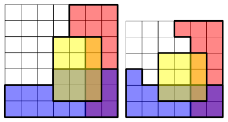
$$P(R, B | Y) = P(R|Y)P(B|Y) \tag{4}\label{4}$$
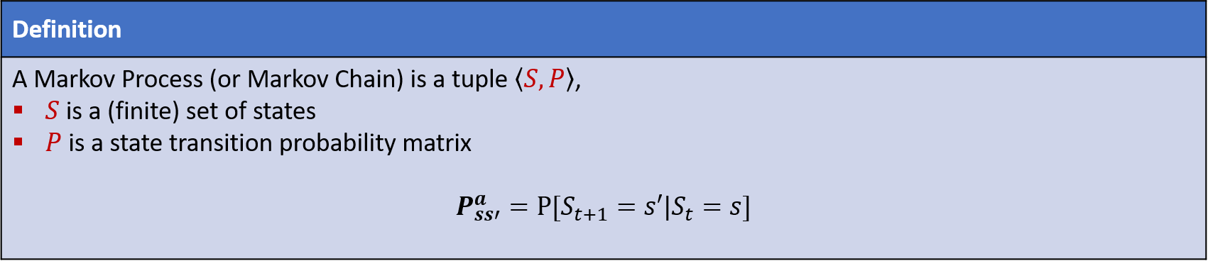
▶ State transitation Matrix
- For a Markov state $s$ and successor state $s'$ , the state transition probability is defined by
$$P_{ss'} = P(S_{t+1}=s' | S_t = s) \tag{5}\label{5}$$
$s$(현재 상태)에서 $s'$(다음 상태)로 이동하는 상태 변환 확률을 식 (5)로 정의한다.
- State transition matrix $P$ defines transition probabilities from all states $s$ to all successor states $s'$, where each row of the matrix sums to 1.

▶ Markov Process (Markov Chains)
- A Markov process is a memoryless random process, i.e. a sequence of random states $S_1, S_2, ... $ with the Markov property.
Markov process는 상대적으로 memory가 덜 필요하는 random process다. (markov property 때문)
random variable, random process, markov process 사이의 관계는 아래와 같은데, markov process는 시간 개념이 들어가 있는 random process의 markov property가 추가된 special case이다. (보다 연산에 있어서 효율적)

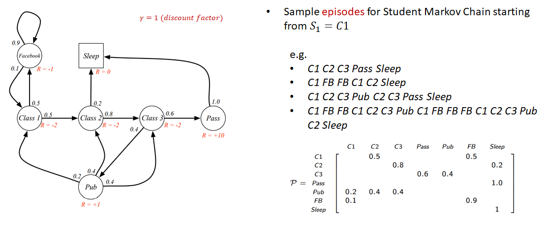
Example : Student Markov Chain
- State
- State transition matrix
주의 : 아래의 화살표가 나타내는 것은 Action이 아닌, state transition 이다. 즉, 어떤 상태에 있을 때 확률적으로 자연스럽게 이동하는 것! (아직 action에 대한 것은 언급하지 않았음)

예를 들면, "Class 1"에 있을 때, state transition probability에 의해 0.5의 확률로 "Class 2"로 이동할 수 있다.
2. Markov Reward Processes (MRPs)
▶ Markov Reward Process (Markov Chains)
- A Markov reward process is a Markov chain with values.
MRPs(Markov reward Process)는 Markov Process에 value(Reward, 보상) 및 discount factor가 추가된 것이다.

Example : Student Markov Reward Processes (MRPs)
- State
- State transition matrix
- Reward function
- Discount factor
예를 들면, "Class 1"에 있을 때, state transition probability에 의해 0.5의 확률로 "Class 2"로 이동하는 경우, Reward 가 -2이다. (state를 떠날때 reward을 받음)
▶ Markov Reward Process (Markov Chains) → Return
강화학습의 목적은 즉각적인 reward에서 끝이 아닌, $t$에서부터 시작해서 끝날때까지 reward가 누적된, 즉 total discount reward를 최대로 하는 것이다. 이를 $G_t$라고 부르며, 정의는 다음과 같다.
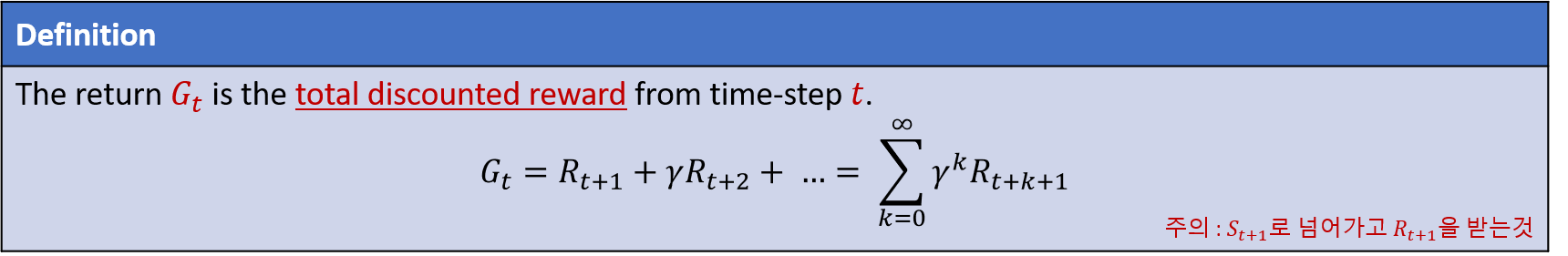
주의 : $R_{t+1}$은 $S_{t+1}$로 넘어가서 $R_{t+1}$을 받는 것이다.
종종 다른 교재 및 참고서에서는 $R_t$로 표기되기도 하는데, 여기서는 $R_{t+1}$로 약속한다. (의미는 같음)
- The discount $\gamma \in [0, 1]$ is the present value of future rewards
- The value of receiving reward $R$ after $k + 1$ time-steps is $\gamma^{k}R$
- This values immediate reward above delayed reward.
Example : Student MRP Returns
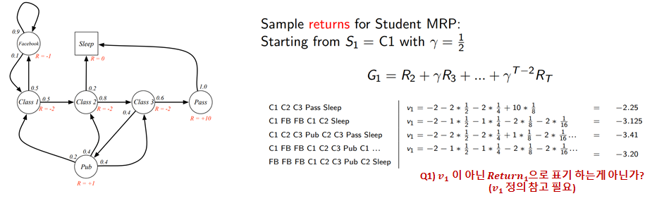
$C_1$부터 종료지점인 Sleep까지의 Return은 여러 case가 존재할 것이다. (위의, 예제에서는 4개의 case의 return을 계산한 결과다.)
Q1) 위에서 Return을 $v_1$으로 표기하였는데, $G_{1}$ (Return) 라고 해야할것 같습니다.
▶ Markov Reward Process (Markov Chains) → Return → Why discount?
Most Markov reward and decision processes are discounted. Why?
대부분의 MRP, MDP는 discount facor가 1이 아닌 미래의 보상을 감소시키는 값을 선택한다. 그 이유는 무엇일까?
- Mathematically convenient to discount rewards
- Avoids infinite returns in cyclic Markov processes
- Uncertainty about the future may not be fully represented
- If the reward is financial, immediate rewards may earn more interest than delayed rewards
- Animal/human behaviour shows preference for immediate reward
- It is sometimes possible to use undiscounted Markov reward processes (i.e. $\gamma = 1$), e.g. if all sequences terminate.
▶ Markov Reward Process (Markov Chains) → Value function
- The value function $v(s)$ gives the long-term value of state $s$.
value function은 현재 내가 있는 $S_t$에서의 가치는 얼마인가? 질문에 정량적인 값을 답을 해주며, 이는 상태 $s$로부터 시작하여 episode가 끝날 때 까지 얻는 Return ($G_t$) (discounted cummulative reward)의 기댓값!


value function을 전개하면 다음과 같다.

Example : State-Value function for student MRP (1)

- $\gamma = 0$일 때, $v_{pub}$을 계산해보자.
$$v_{pub} = 1 + 0 \times [(0.2 \times -2) + (0.4 \times -2) + (0.4 \times -2)] = 1$$
Example : State-Value function for student MRP (2)

- $\gamma = 0.9$일 때, $v_{pub}$을 계산해보자.
$$v_{pub} = 1 + 0.9 \times [(0.2 \times -5) + (0.4 \times 0.9) + (0.4 \times 4.1)] = 1.9$$
Example : State-Value function for student MRP (3)

- $\gamma = 1$일 때, $v_{pub}$을 계산해보자.
$$v_{pub} = 1 + 1 \times [(0.2 \times -13) + (0.4 \times 1.5) + (0.4 \times 4.3)] = 0.8$$
▶ Markov Reward Process (Markov Chains) → Bellman Equation for MRPs (1)
The value function can be decomposed into two parts :
- immediate reward $R_{t+1}$
- discounted value of successor state $\gamma v(S_{t+1})$
결론적으로 말하면, value function은 아래와 같이 two parts로 분해할 수 있다. (이런 꼴을 Bellman Equation이라고 부름)

위 식이 당연하게 보일지도 모르지만, 마지막 부분을 도출하는 과정은 중간과정이 생략되어 있다. 이를 반드시 집고 넘어가는게 좋을것 같아. 아래 정리를 하도록 하겠다.
하지만, 확률에 대한 개념인 기댓값, 조건부 확률의 기댓값, iterated expectation에 대해 사전 지식이 필요하므로 step 1(expectation, conditional expectation) 및 step 2(iterated expectation), step 3 를 먼저 다루고자 한다.

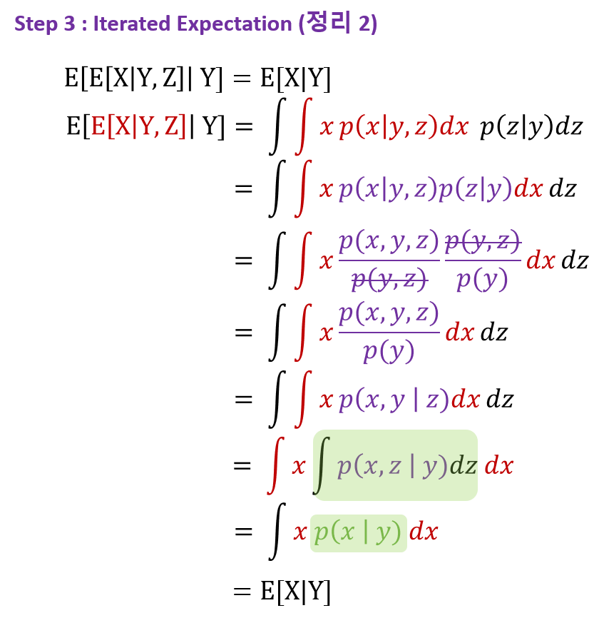
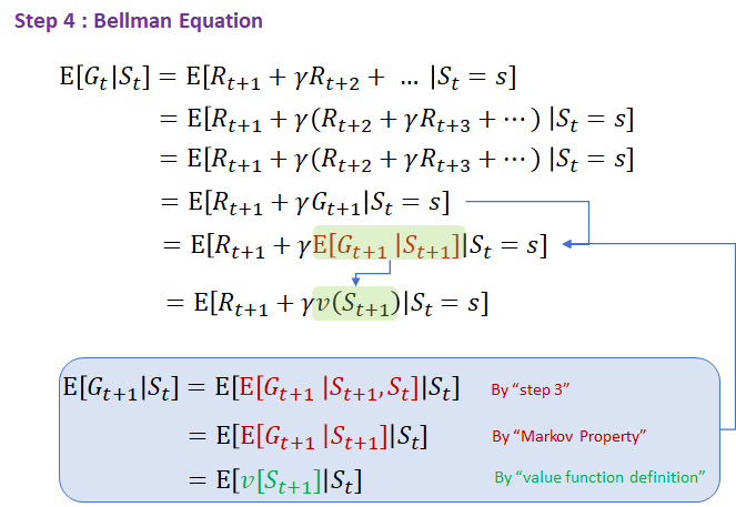
위 step 3의 정리를 가지고 value function에 적용하면 새로운 value function을 $v$에 대해 recursive하게 만들 수 있으며, 이를 Bellman Equation for MRPs 라고 부른다.
즉, Bellman expectation equation은 현재 상태의 가치함수 $V(s_{t})$와 다음 상태의 가치함수 $V(s_{t+1})$ 사이의 관계를 말해주는 방적이다. 강화학습은 벨만 방정식을 어떻게 풀어가느냐가에 따라 다양한 알고리즘이 존재합니다.
Q2) 위에서 Return을 $G_{t+1}$에서 $E[G_{t+1}|S_{t+1}]$로 변경되었는데, 뭔가 부자연스러워 다시 풀어보기
A2) ...
강조 : value function를 Bellman Equation로 만든 위 식의 전개과정 및 암기 필수.
▶ Markov Reward Process (Markov Chains) → Bellman Equation for MRPs (2)
아래 그림을 "backup diagram"이라고도 부른다.

▶ Markov Reward Process (Markov Chains) → Bellman Equation → Bellman Equation in Matrix Form
- The Bellman equation can be expressed concisely using matrices where $v$ is a column vector with one entry per state
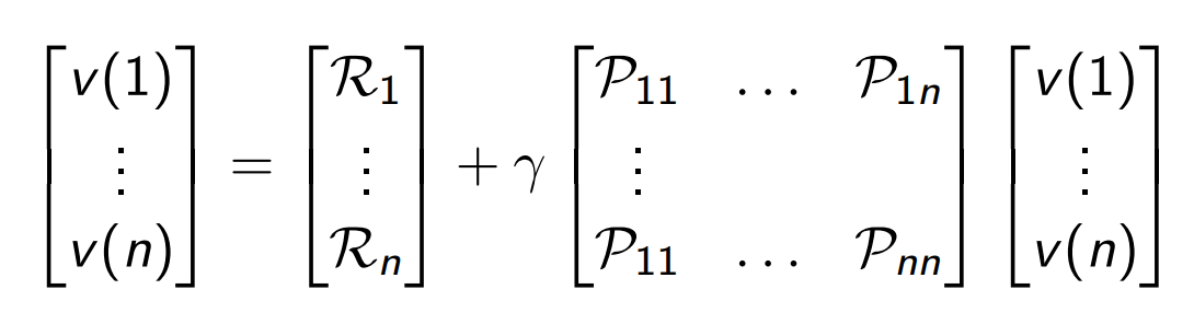
▶ Markov Reward Process (Markov Chains) → Bellman Equation → Solving the Bellman Equation
- The Bellman equation is a linear equation
- It can be solved directly
$$
\begin{aligned}
v &=\mathcal{R}+\gamma \mathcal{P} v \\
(I-\gamma \mathcal{P}) v &=\mathcal{R} \\
v &=(I-\gamma \mathcal{P})^{-1} \mathcal{R}
\end{aligned}
$$
- Computational complexity is $O(n^3)$ for $n$ states
- Direct solution only possible for small MRPs
- There are many iterative methods for large MRPs, e.g.
- Dynamic programming (Ch3 내용)
- Monte-Carlo evaluation (Ch4, model free)
- Temporal-Difference learning (Ch4, model free)
지금까지 model-based인, State, State transition probability, Return(Reward), Discount factor로 구성된 MRP를 살펴보았다. 다음 시간에는 Action이 추가된 MDP에 대해 알아보고자 한다.
Reference
'Reinforcement Learning (d.silver)' 카테고리의 다른 글
| 2.3 The 10-armed Testbed (0) | 2020.07.24 |
|---|---|
| 2.2 Action-value Methods (0) | 2020.07.24 |


댓글