[Paper Review] MULTI-SCALE CONTEXT AGGREGATION BY DILATED CONVOLUTIONS

[Abstract]

 

Contents

---

• Introduction
• Dilated convolutions
• Multi-Scale context aggregation
• Front-End
• Experiments
• Conclusion

 

Keywords

---

• Image Segmentation, Dilated convolutions

 

Introduction

---

• Computer vision에서 다루는 많은 문제들은 instances of dense prediction 이며, 목적은 이미지의 각 픽셀에 대해 연속/불연속 label을 계산하는 것이다. (Example : semantic segmentation (classifying each pixel into one of a given set of categories)
• semantic segmenation은 pixel-level의 정확도와 multi-scale contextual을 결합해야하므로 어려운 점이 있음 (?)

 

• 최근 backpropagation에 의해 훈련된 convolution networks를 통해 semantic segmenation 분야에서의 상당한 정확도를 얻었음
• 구체적으로, "Long et al. 2015"에서는 원래 이미지 분류를 위해 개발된 convolution network architectures를 조금 변경하여 dense prediction을 할 수 있다는 연구를 보여주고 있음
• 이러한, 네트워크는 기존 semantic segmentation challenging의 SOTA 보다 좋은 성능을 보였으며,
• 위의 결과가 image clssification과 dense prediction 사이의 구조적 차이에 의해 동기 부여 된 아래 두 가지 궁금증을 만들었다고 한다.

1. Which aspects of the repurposed networks are truly necessary and which reduce accuracy when operated densely?
2. Can dedicated modules designed specifically for dense prediction improve accuracy further?

 즉, 첫째, semantic segmentaion을 위한 네트워크 구조의 어떤 측면이 필요로 하는지, 그리고, densely하게 계산될때 정확도를 감소시키는지, 둘째, dense prediction을 위해 설계된 module이 정확도를 더욱 향상 시킬 수 있는지? 에 대한 궁금증을 만들었다고 한다. (확인 필요)

•  image classification에서의 network는 연속적으으로 해상도를 줄이는 pooling 및 sub-sampling의 layer들을 지나면서 global prediction을 얻고, multi-scale contextual information을 통합한다.
•  image classification과 대조적으로, dense prediction의 network는 전체 해상도 출력과 결합된 multi-scale 추론 을 요구한다. 
• 최근 "multi-scale 추론" 과 "full-resolution dense prediction"의 상충되는 요구를 처리하기 위한 두 가지 접근법을 연구했다. 

1. One approach involves repeated up-convolutions that aim to recover lost resolution while carrying over the global perspective from downsampled layers (This leaves open the question of whether severe intermediate downsampling was truly necessary.)
2. Another approach involves providing multiple rescaled versions of the image as input to the network and combining the predictions obtained for these multiple inputs. (Again, it is not clear whether separate analysis of rescaled input images is truly necessary.)

•  본 논문에서는 해상도를 잃거나 크기가 조정 된 이미지를 분석하지 않고, multi-scale contextual information을 모을 수 있는 CNN module을 만들었다. 

... 작성중 날아감

 

DILATED CONVOLUTIONS

---

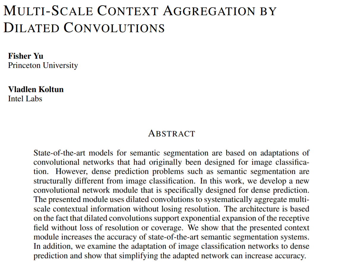
• $F : \mathbf{Z}^2 \rightarrow \mathbf{R}$ be a discrete function
• $\Omega_{r}=[-r, r]^{2} \cap \mathbb{Z}^{2}$
• $k: \Omega_{r} \rightarrow \mathbb{R}$ be a discrete filter of size $(2r+1)^2$
• $*$ : The discrete convolution operator [Figure 1]의 left 식
• $*_{l}$ : a dilated convolution or an $l$-dilated convolution. ($l$ : a dilation factor) [Figure 2]의 right 식

[Figure 1] Standard Convolution (Left), Dilated Convolution (Right)

• Example of 2D Convolution

Example of 2D Convolution

 위 수식이 직관적이지 않기 때문에(제 기준), 아래 animation을 보면 이해하기 수월함

When l = 1, it is standard convolution.	When l = 2, it is dilated convolution.

• 위 그림을 통해서 size가 동일한 kernel(parameters = 9)을, $l = 2$일 때, $l=1$ 보다, convolution을 통해 얻어진 feature map의 커버할 수 있는 the receptive filed가 더 넓은 것을 확인할 수 있다. 

 

[Figure 2] 동일한 input에 대한 standard convolution / atrous convolution 비교

 정보의 양이 늘어나게 된다면, 자연스럽게 모델의 성능은 좋아질 것이다. 하지만, 학습해야 할 양이 많아서 연산량이 증가하게 되는 문제점 및 overfitting 문제점이 존재함. 이처럼 Receptive field(정보의 양)의 영역을 넓히기 위해 기존에는 아래와 같은 기법들이 있었다. (이외에 다른 방법들도 존재함)

• filter의 크기 ↑
• layer 갯수 ↑
• pooling 사용 (그러나, Poling의 경우 연산량 까지 감소할 수 있지만 정보의 손실 발생)

 하지만, 이 논문에서의 제안하고 있는 Dilated Convolution는 Receptive field를 크게 만들어 커버하는 영역을 크게 만들면서, filter의 크기는 동일하게하여, 연산량의 증가는 가져오지 않는 효과적인 방법이다. 보다 구체적으로 아래의 [Figure 3]을 보면서 확인해보자.

[Figure 3] Systematic dilation supports exponential expansion of the receptive field without loss of resolution or coverage.

• (a) : $F_0$ (receptive filed, green) → "3x3 filter with 1-dilated convolution" (parameter 9개, red points) → $F_1$
• (b) : $F_1$ (receptive filed, green)→ "3x3 filter with 2-dilated convolution, padding 1" (parameter 9개, red points) ≒ 7x7 filter → $F_2$
• (c) : $F_2$ (receptive filed, green)→ "3x3 filter with 4-dilated convolution, padding 3" (parameter 9개, red points) ≒ 15 x 15 filter → $F_3$

9 개의 parameter를 가지고도 $l \gt 1$ dilated convolution을 사용하면, 각각 더 큰 filter(kernel)와 동일한 시야를 가진다. 

• parameter가 갯수가 linearly하게 증가하지만, receptive-filed는 exponentially으로 증가하므로, 상대적으로 dilated convolution은 효율적
• $i$에 따라서, receptive filed의 size는 아래와 같이 지수적 증가!

$$
F_{i+1} \text { is }\left(2^{i+2}-1\right) \times\left(2^{i+2}-1\right) \tag{1}\label{1}
$$

 

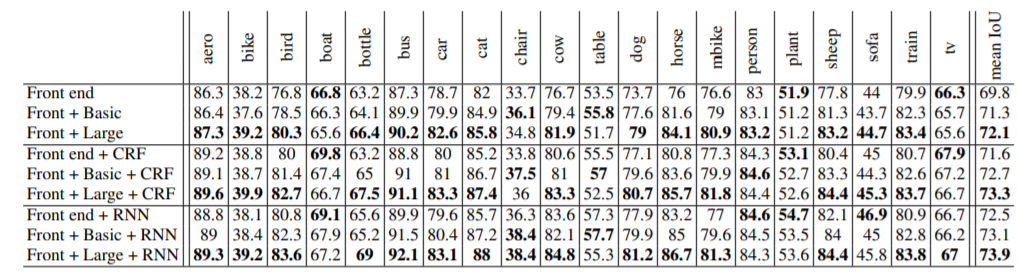
MULTI-SCALE CONTEXT AGGREGATION

---

• Context module : multi-scale contextual information을 집계하여 dense prediction 구조의 성능을 높이기 위함
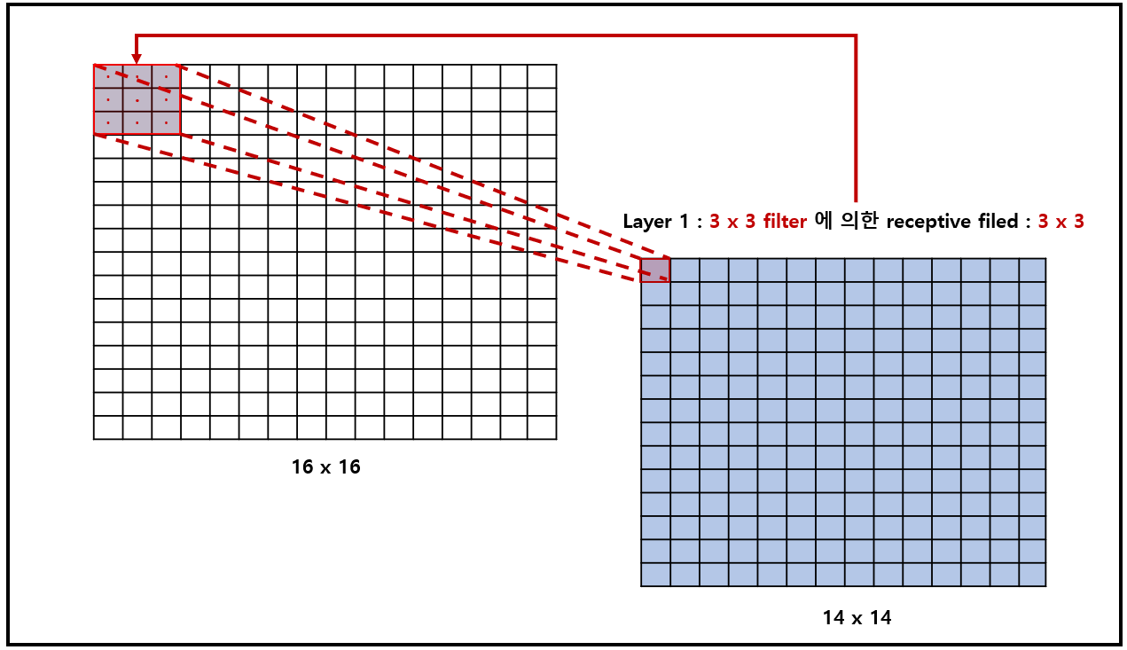
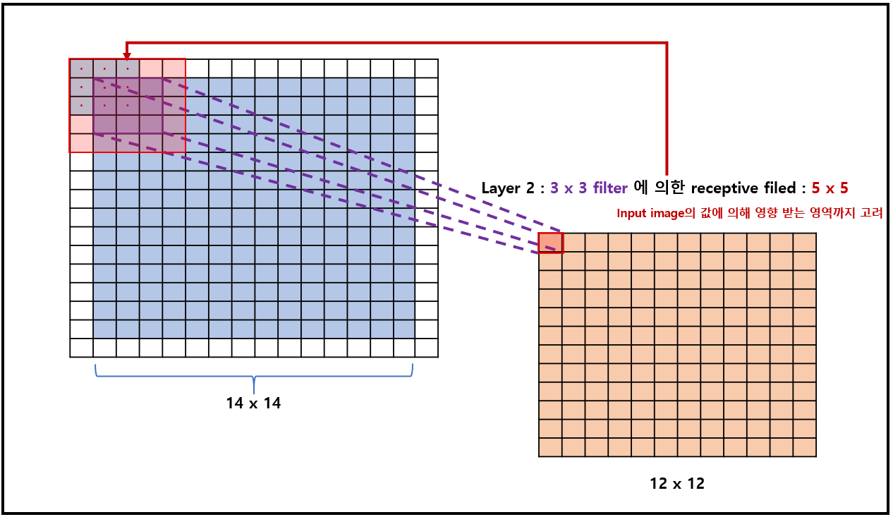
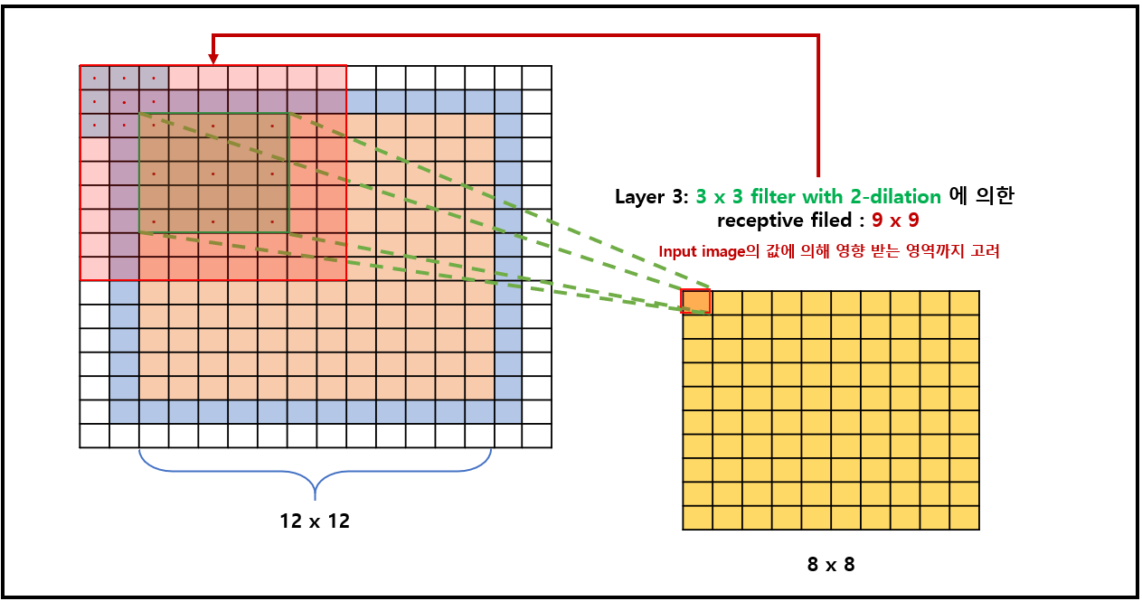
• input of context module : font-end(e.g. vgg16)를 통해 해상도가 64x64의 feature map 
• Layer 1 ~ Layer 7 : 3x3 convolution with diffrent dilation
• Layer 8 : 1x1 convolution with 1-dilation
• truncation : colvolution 이후에 activation function을 ReLU 사용

[Figure 4] Table 1: Context network architecture.

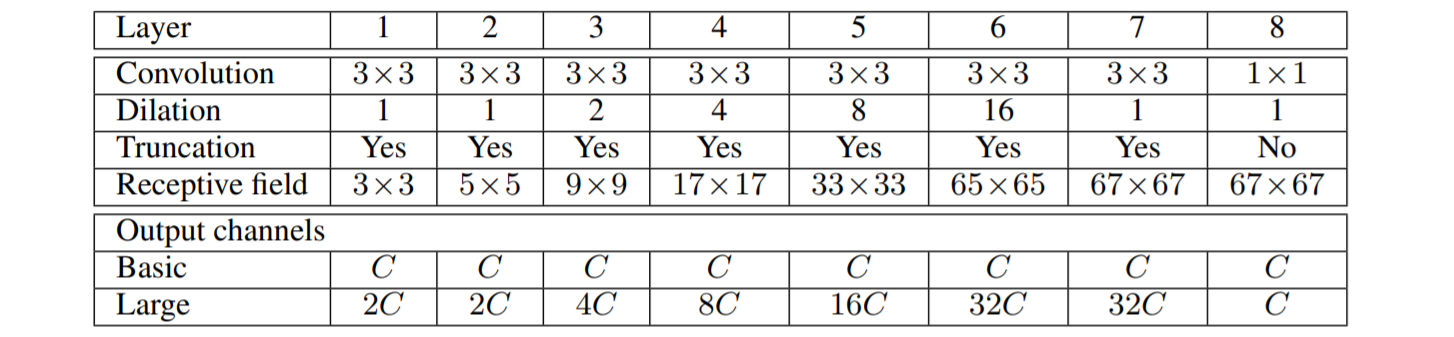
Receptive field : Layer를 지날때, convolution (kernel의 size 및 dilation 설정)에 따라 receptive filed의 size는 다름을 주의

Layer 1에 대한 receptive filed : 3x3	Layer 2에 대한 receptive filed : 5x5
Layer 3에 대한 receptive filed : 9x9

• Context module을 구성하고 있는 Layer의 weight를 standard initialization (CNN에서는 주로 samples from random distribution)진행 후, 학습시켰더니 학습 실패...
• alternative initialization with clear semantics to be much more effective : identity initialization

basic in context module

$$
k^{b}(\mathbf{t}, a)=1_{[\mathbf{t}=0]} 1_{[a=b]} \tag{2}\label{2}
$$

where

• $a$ : the index of the input feature map
• $b$ : the index of the output map.

Large in context module

$$
k^{b}(\mathbf{t}, a)=\left\{\begin{array}{cl}
\frac{C}{c_{i+1}} & \mathbf{t}=0 \text { and } \quad\left\lfloor\frac{a C}{c_{i}}\right\rfloor=\left\lfloor\frac{b C}{c_{i+1}}\right\rfloor. \\
\varepsilon & \text { otherwise }
\end{array}\right.
$$

where

• $\varepsilon \sim N(0, \sigma^2)$
• $\sigma \lt C / c_{i+1}$

 

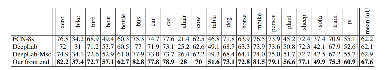
Front  END

---

• a front-end prediction module : VGG-16 network for dense prediction
• 마지막 두개의 layer에 존재하는 pooing 및 striding 제거 (확인 필요)
• 마지막 layer를 제외한 모든 layer의 convolution 연산은 2-dilated 적용
• 마지막 layer의 convolution 은 4-dialted 적용
• convolution을 바꾸면서 기존 학습된 weight를 모두 초기화시켜야 했지만, 고해상도의 output을 얻을 수 있다.

Q&A (2) : We use reflection padding : the buffer zone is filled by reflecting the image about each edge. 

Answer :

Padding of 1 adds an extra layers on top of the input matrix. Left: Zero padding. Middle: Reflection padding. Right: Replication padding

▶ Trainning

• SGD
• minibatch size : 14
• learning rate : $10^{-3}$
• momentum : 0.9
• iteration : 60K

[Figure 5] Semantic segmentations produced by different adaptations of the VGG-16 classification network.

[Figure 6] Our front-end prediction module is simpler and more accurate than prior models. This table reports accuracy on the VOC-2012 test set.

 

EXPERIMENTS

---

[Figure 7] Semantic segmentations produced by different models.

[Figure 8] Controlled evaluation of the effect of the context module on the accuracy of three different architectures for semantic segmentation.

 

[Figure 9] Evaluation on the VOC-2012 test set. ‘DeepLab++’ stands for DeepLab-CRF-COCO-LargeFOV and ‘DeepLab-MSc++’ stands for DeepLab-MSc-CRF-LargeFOV-COCO-CrossJoint (Chen et al., 2015a).

 

CONCLUSION

---

...

 

 

References

---

• Review: DilatedNet — Dilated Convolution (Semantic Segmentation)
• MULTI-SCALE CONTEXT AGGREGATION BY DILATED CONVOLUTIONS
• receptive field(수용영역, 수용장)과 dilated convolution(팽창된 컨볼루션)