2020-2학기 이화여대 김정태 교수님 강의 내용을 바탕으로 본 글을 작성하였습니다.
Overview
- Curve fitting
- Probability theory
- Curve fitting revisited
- Bayesian curve fitting
Curve fitting problem
ML에서 중요한 개념들에 대한 통찰력있는 직관을 가져보기 위해 간단한 회귀 문제(Regression)를 생각해보자.
- We observe a real value input $x$ and wish to use this observation to predict the value of a real valued target value $t$.
- We have our training data $\mathbf{x} = (x_1, ..., x_N )^{T}$ and $t = (t_1, ..., t_N )^T$.
- Our goal is to exploit this training data set in order to make predictions of the value $\hat{t}$ for some new value $\hat{x}$.
- Uncertainties exist because there is observation noise and the amount of available data is finite.
- Probability theory provides a framework for expressing uncertainty and decision theory exploit the representation to make optimal predictions.
불확실성이 존재하는 두 가지 이유는 다음과 같다. 첫째, 관측 데이터 자체의 noise 때문에 발생, 둘째, 사용 가능한 데이터의 양이 유한하기 때문이다. 불확실성을 수학적으로 표현하고, 최적의 회귀 모델을 결정하는데 필요한 도구가 확률 이론이다.
Example : Polynomial curve fitting
$M$ 차 다항식 함수를 사용하여 데이터를 맞추는 간단한 접근 방식으로 아래 (1)식을 생각할 수 있다.
$$y (x, \mathbf{w}) = \sum_{j=0}^{M} w_j x^j \tag{1}\label{eq1}$$
where $\mathbf{w} = (w_0, ... , w_M)$.
- The values of the coefficients will be determined by fitting the polynomial to the training data, which is done by minimizing an error function that measures the mismatch between the function $y(x, \mathbf{w})$ for any givven value $\mathbf{w}$ and the training data set
- We have our training data $\mathbf{x} = (x_1, ..., x_N )^{T}$ and $t = (t_1, ..., t_N )^T$.
- Our goal is to exploit this training data set in order to make predictions of the value $\hat{t}$ for some new value $\hat{x}$.
Error function
Error function(오차 함수)을 아래 식 (2)로 정의하고, 이를 가능한 최소화함으로써 적당한 $\mathbf{w}$를 찾아야 한다.
$$ E(\mathbf{w}) = \frac{1}{2} \sum_{n=1}^{N} \{y(x_n, \mathbf{w}) - t_n \}^2 \tag{2}\label{eq2}$$
- Because the error function is a quadratic of $\mathbf{w}$, its gradient is linear, so the minimization problem can be solved analytically and the solution is unique, which is extremely exceptional.

Model comparison or model selection
오차 함수를 통해 적절한 $\mathbf{w}$를 찾을 수 있었다면, 나머지 남은 일은 다항식의 $M$(차수)을 결정해야하는 것이다. 아래 식 (3) 인 $E_{RMS}$을 통해 적합한 model selection을 해야함.
- There remains problem of choosing the order $M$ of the polynomial.
- Constant or first order polynomial give rather poor fit to the data.
- Third order seems to give the best fit to the function of sin(2$\pi x$).
- To measure the performance of the fitting system, we measure root mean square error (RMSE)for both training and test data set.
$$E_{RMS} = \sqrt{2E(\mathbf{w}^{*}/N)} \tag{3}\label{eq3}$$
Overfitting
- Although we obtain an excellent fit to the data as we go to a higher order polynomial ($M = 9$), the fitted curve poorly represents the true function, which is known as overfitting.
궁극적인 목표는 아래 Figure 1.4 의 녹색라인에 가장 가까운 curve를 그리는 것이다. train error도 잘 살펴봐야하지만, 반드시, test error에 관심을 가져야 한다. test error를 확인하지 않는다면 overfitting 문제를 피할 수 없다. $M=3$인 경우, train error는 높지만, test error는 낮을 것이다.

What is happening?
- It may look paradoxical since a polynomial of given order contains all lower order polynomials as special cases.
- The $M = 9$ polynomial is capable of generating results as good as $M = 3$ polynomial
- Moreover based on Taylor series, we know that $M = 9$ polynomial can represent sin(2$\pi x$) better than $M = 3$ polynomial
- However, what is happening is that more flexible polynomial ($M = 9$) fits the data with noise perfectly with coefficients of large magnitudes
Q 1) $M=9$인 경우, $M=3$인 경우를 포함하고 있기 때문에, 그리고 Taylor series에 의하면 다항식의 차수가 높을 수록 더 근사할 수 있는데, 왜 $\mathbf{w^{*}}$를 찾지 못했는가? (즉, 결과가 더 좋지 않은가)
A 1) Figure 1.4 의 training data points들은 noise가 들어가 있는데, $M=9$인 경우 불확실한 noise 까지 fitting하는 학습을 했기 때문이다.

Overfitting을 해결하기 위한 방법은 무엇일까?
- Data augmentation
- Regularization + Validation
- Bayesian approach
- ...
Data augmentation (학습 데이터 증폭/증가)
Data augmentation은 Overfitting을 막기 위해 가장 좋은 방법이지만, 데이터를 구하지 못하는 환경이라면 현실적으로 매우 제한이 있는 방법이다.
- It is interesting to see that the over-fitting problem becomes less severe as the size of the data set increases
- Therefore, data augmentation can be a good way to fight with over-fitting problem
- One heuristic approach is that the number of data point should be no less than some multiple of the number of parameters in the model

Regularization
Regularization은 Overfitting을 막기 위한 또 다른 방법으로, Overfitting이 일어난다면 $\mathbf{w}$(가중치)가 커지는 현상을 이용함으로써 이를 줄여주기 위해 penalty를 도입하여 Overfitting을 극복하는 방안이다.
- Complexity of model should follow the complexity of task, not the size of available data (의미 : 모델의 복잡도를 결정하는데, data 갯수로 판단하면 안된다.)
- Instead of maximum likelihood approach, one may use Bayesian approach to avoid over-fitting problem. (추후 다룰 예정)
- Regularization involves adding a penalty term to the error function in order to discourage the coefficients from reaching larger value
- Weight decay regularization is one popular choice in machine learning
$$ E(\mathbf{w}) = \frac{1}{2} \sum_{n=1}^{N} \{y(x_n - \mathbf{w}) - t_n \}^2 + \frac{\lambda}{2} {||\mathbf{w}||}^2\tag{4}\label{eq4}$$
Regularization 원리
- Overfitting이 일어나면 "weight" 가 크게 설정된다. (Table 1.1 참고 차수가 매우 높아져도 같은 현상)
- 위 문제를 해결하고자 Error function에 penalty를 도입

Regularization parameter

- The minimizer with weight decay regularization is also computed in closed form since the penalty function is also quadratic
- Too large regularization parameter yields poor fit


적당한 penalty parameter를 찾기 위해서는 학습데이터인 train set 이외에 validation set을 구성하여 검증하는 방법이 있다. (주의 : 반드시 train set, validation set, test set은 겹치지 말아야함)
Validation
목적 : test error를 줄이기 위한 hyperparameter인 적당한 $\lambda$를 찾기 위한 방법
- The impact of regularization term by plotting the RMS error in both training and test sets
- One easy way of determining $\lambda$ is using validation data set
- Since it is wasteful to reserve some data for validation, more sophisticated methods have been studying

Probability theory
Define probability of an event by the fraction of times that the event occur out of the total number of trials, in the limit that the total number of trials go to infinity.
Frequentist probability
- The probability of $X$ will take value $x_i$ and $Y$ will do $y_j$ :
$$P(X = x_i , Y = y_j) = \frac{n_{ij}}{N} \tag{5}\label{eq5}$$
- $P(X = x_i)$ 를 marginal probability 라고 부름 (sum rule of probability)
$$P(X =x_i) = \frac{c_i}{N} = \sum_{j=1}^{L} P(X = x_i, Y = y_J) \tag{6}\label{eq6}$$

Conditional probability and Bayes theorem
- The probability of $Y = y_j$ given $X = x_i$ : (conditional probabaility)
$$P(Y=y_j | X = x_i) = \frac{n_{ij}}{c_i} \tag{7}\label{eq7} $$
- The probability of $X$ will take value $x_i$ and $Y$ will do $y_j$ : (joint probability)
$$P\left(X=X_{i}, Y=y_{j}\right)=\frac{n_{i j}}{N}=\frac{n_{i j}}{c_{i}} \frac{c_{i}}{N}=p\left(Y=y_{j} \mid X=x_{i}\right) p\left(X=x_{i}\right) \tag{8}\label{eq8}$$
- The rules of probability (sum rule, product rule)
$$p(X) = \sum_Y p(X, Y) \tag{9}\label{eq9}$$
$$p(X, Y) = p(Y, X) = p(Y|X)p(X) = p(X|Y)p(Y) \tag{10}\label{eq10}$$
- Bayes theorem
$$p(Y|X) = \frac{P(X|Y)p(Y)}{p(X)} \tag{11}\label{eq11}$$
확률과 관련된 자세한 설명은 Probability Theory 를 참고
Bayesian probability
- For certain events, it is difficult to apply the frequentist interpretation of probability. For example, the probability of of Arctic ice cap will disappear.
- In Bayesian viewpoint, probability of an event represents uncertainty or degree of belief about the event. Therefore, we may apply Bayesian probability for many events that are not certain.
- For example, in curve fitting problem, it is difficult to interpret $\mathbf{w}$ as a random variable in frequentist view point but is possible to describe the uncertainty in the parameter in Bayesian view point
- Posterior probability can be viewed by the change of belief after observing the data $D$
$$p(\mathbf{w} | D) = \frac{P(D|\mathbf{w})p(\mathbf{w})}{p(D)} \tag{12}\label{eq12} $$
- Bayes theorem can be described in word by
$$posterior ∝ likelihood \times prior $$
- In a frequentist setting, $\mathbf{w}$ is considered a fixed parameter while it is considered a random variable with a distribution in Bayesian setting
- Bayesian setting can incorporate prior knowledge smoothly while frequentist setting depends only data
- It is important to define proper prior distribution in Bayesian setting
Curve fitting re-visited
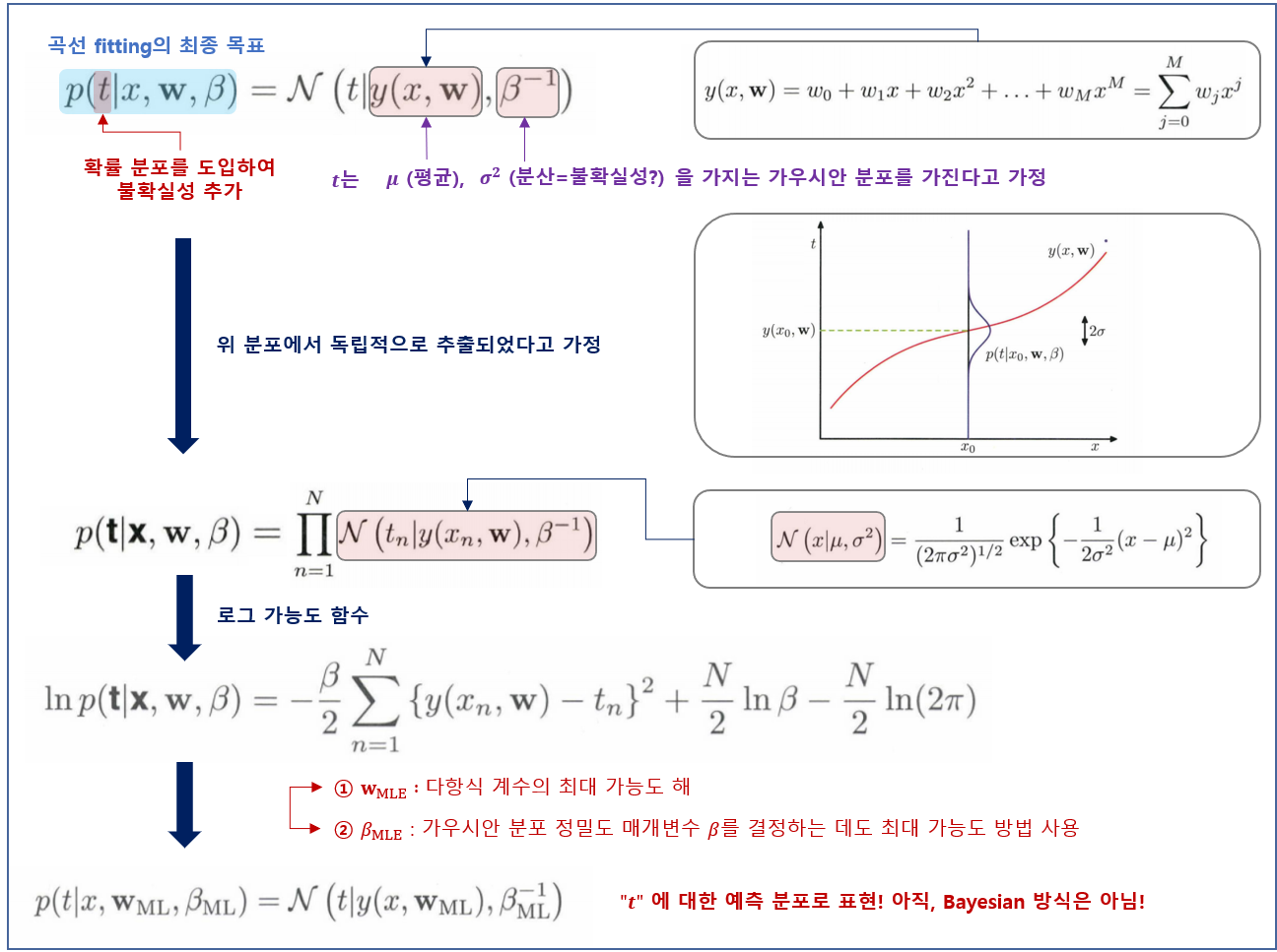
앞에서 다항식 곡선 피팅 문제를 Error function의 측면에서 살펴보았다. 여기서는 같은 곡선 피팅 문제를 확률적 측면에서 살펴봄으로써 Error function과 regularization에 대한 통찰을 얻을 수 있을 것이다. 또한 이는 베이지안 해결법을 도출하는데 도움을 줄 것이다.
아래와 같이 확률 분포(가우시안 분포)를 이용해서 타깃 변수의 값에 대한 불확실성을 표현할 수 있다.
We assume that the distribution of $t$ given $x$ follows Gaussian distribution
$$\left.p(t \mid x, \mathbf{w}, \beta)=\mathcal{N}(t \mid y(x, \mathbf{w}), \beta^{-1}\right) \tag{13}\label{eq13}$$
- mean(평균) : $y(x, \mathbf{w}) = \sum_{j=0}^{M} w_j x^j$
- variance(분산) : $\beta^{-1}$ ($\beta$ : precision parameter)

$x$가 주어졌을 때 $t$의 가우시안 분포, 분포의 평균은 다항 함수 $y(x, \mathbf{w})$로 주어지며, precision(정밀도)는 매개변수 $\beta$로 주어진다. $\beta^{-1} = \sigma^2$ 이다.
이제 훈련 집합 $\{\mathbf{x}, \mathbf{t}\}$를 바탕으로 최대 가능도 방법(MLE)을 이용해서 알려지지 않은 $\mathbf{w}$와 $\beta$를 구해보자. 만약, 데이터가 (식 13)의 분포에서 독립적으로 추출되었다고 가정하면, likelihood function은 다음과 같이 주어질 것이다.
$$p(\mathbf{t} \mid \mathbf{x}, \mathbf{w}, \beta)=\prod_{n=1}^{N} \mathcal{N}\left(t_{n} \mid y\left(x_{n}, \mathbf{w}\right), \beta^{-1}\right) \tag{14}\label{eq14}$$
Log-likelihood function
$$\ln p(\mathbf{t} \mid \mathbf{x}, \mathbf{w}, \beta)=-\frac{\beta}{2} \sum_{n=1}^{N}\left\{y\left(x_{n}, \mathbf{w}\right)-t_{n}\right\}^{2}+\frac{N}{2} \ln \beta-\frac{N}{2} \ln (2 \pi) \tag{15}\label{eq15}$$
- $\mathbf{w}_{MLE}$ : 직접 전개 해보기 (숙제)

즉, 노이즈가 가우시안 분포를 가진다는 가정하에 가능도 함수를 최대화하려는 시도의 결과로 제곱합 오차 함수를 유도할 수 있다.
- $\beta_{MLE}$ : 직접 전개 해보기 (완료)

매개변수 $\mathbf{w}$와 $\beta$를 구했으니, 이제 이를 바탕으로 새로운 변수 $x$에 대해 예측값을 구할 수 있다. 이제 확률 모델을 사용하고 있으므로 예측값($t$)은 전과 같은 점 추정값이 아닌 $t$에 대한 예측 분포로 표현될 것이다. 위에서 얻은 $\mathbf{w}_{MLE}$와 $\beta_{MLE}$를 식 13에 대입하면 다음을 얻을 수 있다.
$$p\left(t \mid x, \mathbf{w}_{\mathrm{ML}}, \beta_{\mathrm{ML}}\right)=\mathcal{N}\left(t \mid y\left(x, \mathbf{w}_{\mathrm{ML}}\right), \beta_{\mathrm{ML}}^{-1}\right) \tag{16}\label{eq16}$$
지금까지 점 추정값 $t$가 아닌 확률 모델을 도입함으로써 $t$에 대한 예측 분포(predictive distribution)로 표현할 수 있음을 다시 정리하면 아래와 같다.
For Bayesian approach using prior, we define
$$p(\mathbf{w} \mid \alpha)=\mathcal{N}\left(\mathbf{w} \mid \mathbf{0}, \alpha^{-1} \mathbf{I}\right)=\left(\frac{\alpha}{2 \pi}\right)^{(M+1) / 2} \exp \left\{-\frac{\alpha}{2} \mathbf{w}^{\mathrm{T}} \mathbf{w}\right\} \tag{17}\label{eq17}$$
베이지안 방식을 향해 더 나아가기 위해, 다항 계수 $\mathbf{w}$에 대한 식 17의 가우시안 분포를 가진 사전 분포(Prior)를 도입할 것이다.
- $M+1$ : $M$차수 다항식 벡터 $\mathbf{w}$의 원소의 갯수 ($0 \sim M$ 개)
- $\alpha$ : model parameter의 분포를 제어하는 변수들을 hyperparameter (초매개변수)라고 함
베이지안 정리에 따라 $\mathbf{w}$의 사후분포(posterior)는 가능도함수와 사전분포의 곱으로 비례할 것이다.
$$p(\mathbf{w} \mid \mathbf{x}, \mathbf{t}, \alpha, \beta) \propto p(\mathbf{t} \mid \mathbf{x}, \mathbf{w}, \beta) p(\mathbf{w} \mid \alpha) \tag{18}\label{eq18}$$
이제 주어진 데이터에 대해 가장 가능성이 높은 $\mathbf{w}$를 찾는 방식으로 $\mathbf{w}$를 결정할 수 있다. 즉, 사후 분포(식 18)을 최대화하는 방식으로 $\mathbf{w}$를 결정할 수 있으며, 이런 테크닉을 "최대 사후 분포(maximum posterior, MAP)라고 한다. 식 18에서 음의 로그를 취한 뒤 사후 확률의 최댓값을 찾는 것이 아래 식의 최솟값을 찾는 과정과 동일함을 알 수 있다.
$$\frac{\beta}{2} \sum_{n=1}^{N}\left\{y\left(x_{n}, \mathbf{w}\right)-t_{n}\right\}^{2}+\frac{\alpha}{2} \mathbf{w}^{\mathrm{T}} \mathbf{w} \tag{19}\label{eq19}$$
사후 분포를 최대화하는 것이 regularization(정규화) 변수인 $\lambda = \frac{\alpha}{\beta}$로 주어진 정규화된 제곱합 오차 함수를 최소화하는 것과 동일함을 확인할 수 있다.
지금까지 베이지안 정리에 따라서 $\mathbf{w}$의 사전분포$p(\mathbf{w}|\alpha)$와 가능도함수를 도입한 사후 분포(MAP)를 Bayes 테크닉을 이용한 것을 정리하면 다음과 같다.

사전 분포 $p(\mathbf{w}|\alpha)$를 포함시키긴 했지만, 여전히 $\mathbf{w}$에 대한 점 추정(?)을 하고 있으므로, 완벽한 베이지안 방법론을 구사한다고 말할 수 없다고 함, 자세한 내용은 이어서 설명하겠다.
Bayesian curve fitting
- MAP estimation is still a point estimation although it considered prior distribution
- Full Bayesian approach requires integration over all values of $\mathbf{w}$
- We usually are interested in the distribution of prediction (not the distribution of weights)
- The integral is intractable for all most every cases except for some simple example such as curve-fitting
$$p(t \mid x, \mathbf{x}, \mathbf{t})=\int p(t \mid x, \mathbf{w}) p(\mathbf{w} \mid \mathbf{x}, \mathbf{t}) \mathrm{d} \mathbf{w} \tag{20}\label{eq20}$$

과정 상세하게 리뷰예정(추석 연휴기간에 수정 예정)
- 예측 분포의 평균(mean)과 분산(variance)이 $x$에 종속되어 있음
- target 변수의 noise로 인한 예측값 $t$의 불확실성이 $s^2(x)$에 $\beta^{-1}$로 표현되어 있음 (이 불확실성은 이미 (식 13)인 "최대 가능도 예측 분포"에서 표현되었다. 하지만, 위의 variance의 두 번째 항은 $\mathbf{w}$의 불확실성으로부터 기인한 것이며, 베이지안 접근법을 통해 구해진 것
- Bayesian curve fitting can be done analytically.
합성 사인 함수 회귀문제에 대한 예측분포가 아래와 같이 표현되어 있다.

Model selection
- Hyper-parameters such as the order of polynomial and regularization parameter should be selected
- Performance of training is not a good indicator for model selection (학습 데이터의 성능은 의미 없음)
- If data is plentiful, one can use some portion of data for validation
- If model design is iterated many times using a limited size data, over-fitting to validation data can occur
- One may use cross-validation approach, however training is computationally intensive and there exist many hyper-paremters

Bayesian information criteria
- Various information criteria have been proposed that attempt to correct for bias of maximum likelihood by the addition of a penalty term
- Akaike information criterion (AIC) choose the model for which the quantity is maximized
$$\log p(D|\mathbf{w}_{ML}) - M$$
where $M$ is thew number of adjustable parameters
- Bayesian information criterion (BIC) can be used. In practice, the model often prefers simple model
- It is desirable to consider uncertainty in model parameter.
수식 전개 작성부분이 남아 있어 중간에 작성 중에 있습니다.
Reference
- Pattern Recognition and Machine Learning
- PRML Example Code (git) : github.com/ctgk/PRML
'패턴인식과 머신러닝 > Ch 01. Introduction' 카테고리의 다른 글
| [베이지안 딥러닝] Appendix. Calculus of Variations (변분법) (0) | 2021.02.08 |
|---|---|
| [베이지안 딥러닝] Introduction - Decision Theory and Information Theory I (0) | 2020.09.29 |
| [베이지안 딥러닝] Introduction (2) | 2020.09.01 |
| 1.2 Probability Theory (0) | 2020.07.09 |


댓글