2020-2학기 이화여대 김정태 교수님 강의 내용을 바탕으로 본 글을 작성하였습니다.
Ch4.1에서는 분류를 위한 discriminant function을 이용한 접근법을 다뤘으며, 이번 Ch4.2에서는 클래스별 conditional distribution인 $p(\mathbf{x}|C_k)$와 클래스의 prior distribution인 $p(C_k)$를 모델하고, 베이지안 정리를 적용하여 $p(C_k|\mathbf{x})$ (posterior probability)를 계산해 내는 방식의 probabilistic generative models을 사용할 것이다.
Overview
- Linear classification
- Probabilistic generative model
- Probabilistic discriminative model
- The Laplace Approximation
- Bayesian Logistic Regression
Probabilistic Generative Models
▶ Two classes case (sigmoid function)
우선 class가 두 개인 경우를 고려해 보자. class $C_1$에 대한 사후 확률을 식 (1)로 표현할 수 있음
$$
\begin{aligned}
p\left(\mathcal{C}_{1} \mid \mathbf{x}\right) &=\frac{p\left(\mathbf{x} \mid \mathcal{C}_{1}\right) p\left(\mathcal{C}_{1}\right)}{p\left(\mathbf{x} \mid \mathcal{C}_{1}\right) p\left(\mathcal{C}_{1}\right)+p\left(\mathbf{x} \mid \mathcal{C}_{2}\right) p\left(\mathcal{C}_{2}\right)} \\
&=\frac{1}{1+\exp (-a)}=\sigma(a)
\end{aligned} \tag{1}\label{1}
$$
where we have defined
$$a=\ln \frac{p\left(\mathbf{x} \mid \mathcal{C}_{1}\right) p\left(\mathcal{C}_{1}\right)}{p\left(\mathbf{x} \mid \mathcal{C}_{2}\right) p\left(\mathcal{C}_{2}\right)} \tag{2}\label{2}$$
$-\infty \lt a \lt \infty$
▶ The logistic sigmoid function is defined by
그리고 $\sigma(a)$는 logistic sigmoid 함수로 식 (3)으로 정의 및 [그림 1] 빨간 실선으로 그려져 있음
$$\sigma(a) = \frac{1}{1+exp(-a)} \tag{3}\label{3}$$
$ 0 \leq \sigma(a) \leq 1$
Why? class 분류를 하기 위해서 "0~1" 사이의 값을 가지는 사후확률을 구해야함

▶ Symmetry property of logistic sigmoid function (특징)
$$\sigma(-a) = 1 - \sigma(a) \tag{4}\label{4}$$
▶ The inverse of the logistic sigmoid
$$a = \ln(\frac{\sigma}{1-\sigma}) \tag{5}\label{5}$$
식 (5)를 logit function 라고 부르기도 하며, 두 클래스에 대한 확률들의 비율의 로그값인 $\ln[(\frac{p(\mathcal{C_1}|\mathbf{x})}{p(\mathcal{C_2}|\mathbf{x})})]$을 나타낸다. 이를 log odds라 불리기도 함.
▶ If $a(\mathbf{x})$ is a linear function of x, in which case the posterior probability is governed by a generalized linear model.
$a(\mathbf{x})$가 $\mathbf{x}$에 선형 함수인 경우에 추후 살펴볼 것인데, 이때 사후확률은 일반화된 선형 모델에 의해 조절됨. (참고)
▶ Multi classes case (softmax function : normalized exponential function)
$K \gt 2$인 경우는 식 (6)과 같이 된다.
$$
\begin{aligned}
p\left(\mathcal{C}_{k} \mid \mathbf{x}\right) &=\frac{p\left(\mathbf{x} \mid \mathcal{C}_{k}\right) p\left(\mathcal{C}_{k}\right)}{\sum_{j} p\left(\mathbf{x} \mid \mathcal{C}_{j}\right) p\left(\mathcal{C}_{j}\right)} \\
&=\frac{\exp \left(a_{k}\right)}{\sum_{j} \exp \left(a_{j}\right)}
\end{aligned} \tag{6}\label{6}
$$
where
$$a_k = \ln(p(\mathbf{x}|\mathcal{C_k})p(\mathcal{C_k})). \tag{7}\label{7}$$
▶ The normalized exponential is also known as the softmax function, as it represents a smoothed version of the ‘max’ function because, if $a_{k} \gg a_{j}$ for all $j \neq k$, then $p\left(\mathcal{C}_{k} \mid \mathbf{x}\right) \simeq 1$, and $p\left(\mathcal{C}_{j} \mid \mathbf{x}\right) \simeq 0$
식 (6)의 아래항을 보면 정규화된 지수함수가 있으며, 이를 softmax function이라고도 부름,
이제 클래스별 조건부 밀도인 $p(\mathbf{x}|C_k)$에 대해서 특정 형태(gaussian distribution)를 선택했을 경우의 결과에 대해 살펴보도록 하자.
클래스별 조건부 밀도 input에 성질에 따라 아래와 같은 특정 distribution을 적용할 수 있음
- case 1) continious input : (e.g. gaussian distribution)
- case 2) discrete input : (e.g. naive bayes) [이 부분은 생략!]
4.2.1 continious input (연속 입력)
▶ Assume class conditional distribution is Gaussian (parametric model)
$$
p\left(\mathbf{x} \mid \mathcal{C}_{k}\right)=\frac{1}{(2 \pi)^{D / 2}} \frac{1}{|\mathbf{\Sigma}|^{1 / 2}} \exp \left\{-\frac{1}{2}\left(\mathbf{x}-\boldsymbol{\mu}_{k}\right)^{\mathrm{T}} \boldsymbol{\Sigma}^{-1}\left(\mathbf{x}-\boldsymbol{\mu}_{k}\right)\right\} \tag{8}\label{8}
$$
▶ Two classes case
우선, 클래스가 두 개인 경우에 대해 고려해 보면, 식 (1)과 식(2)로부터 다음을 구할 수 있음
$$
p\left(\mathcal{C}_{1} \mid \mathbf{x}\right)=\sigma\left(\mathbf{w}^{\mathrm{T}} \mathbf{x}+w_{0}\right) \tag{9}\label{9}
$$
where
$$
\begin{aligned}
\mathbf{w} &=\boldsymbol{\Sigma}^{-1}\left(\boldsymbol{\mu}_{1}-\boldsymbol{\mu}_{2}\right) \\
w_{0} &=-\frac{1}{2} \boldsymbol{\mu}_{1}^{\mathrm{T}} \boldsymbol{\Sigma}^{-1} \boldsymbol{\mu}_{1}+\frac{1}{2} \boldsymbol{\mu}_{2}^{\mathrm{T}} \boldsymbol{\Sigma}^{-1} \boldsymbol{\mu}_{2}+\ln \frac{p\left(\mathcal{C}_{1}\right)}{p\left(\mathcal{C}_{2}\right)}
\end{aligned} \tag{10}\label{10}
$$

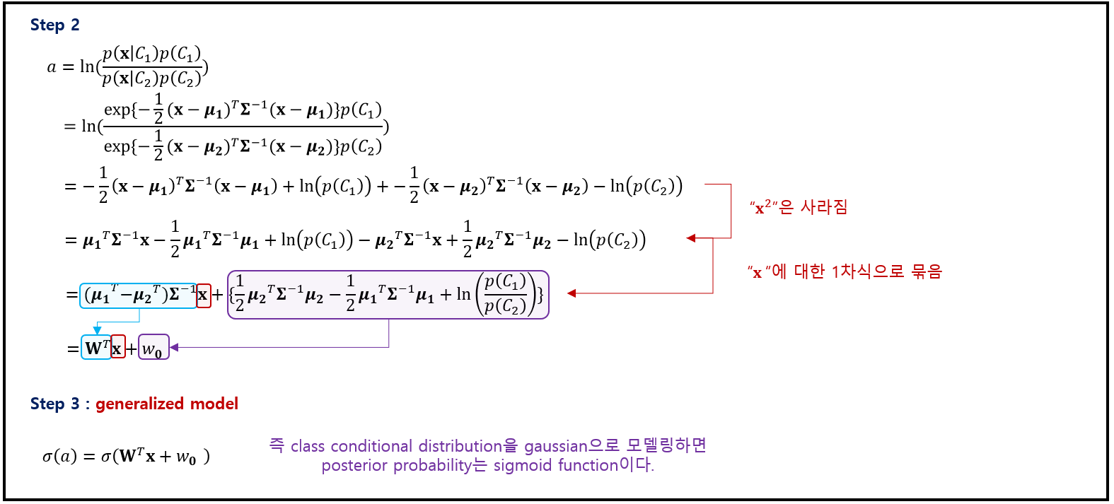
Gaussian distribution의 지수부의 $\mathbf{x}$에 대한 이차항이 사라짐(공분산 같다고 가정했기 때문)으로써 logistic sigmoid function의 입력 변수 $\mathbf{x}$에 대한 선형 함수가 되었음.
추가적으로 2차원 입력 공간의 $\mathbf{x}$의 경우에 대한 sigmoid function은 [그림 2]에 나타내고 있음.

사전확률 $p(C_k)$는 $\omega_0$ (bias)를 통해서만 연관되며, 사전분포를 바꾸는 것은 결정 경계를 평행하게 이동하는 효과를 가짐!
▶ Genearl case of $K$ classes
더 일반적인 $K$개의 클래스 경우에는 식 (6), (7)에 의해 다음과 같게 된다.
$$
a_{k}(\mathbf{x})=\mathbf{w}_{k}^{\mathrm{T}} \mathbf{x}+w_{k 0} \tag{11}\label{11}
$$
where
$$
\begin{aligned}
\mathbf{w}_{k} &=\boldsymbol{\Sigma}^{-1} \boldsymbol{\mu}_{k} \\
w_{k 0} &=-\frac{1}{2} \boldsymbol{\mu}_{k}^{\mathrm{T}} \boldsymbol{\Sigma}^{-1} \boldsymbol{\mu}_{k}+\ln p\left(\mathcal{C}_{k}\right)
\end{aligned} \tag{12}\label{12}
$$
4.2.2 Maximum likelihood solution (최대 가능도 해)
4.1.1에서 다룬 class conditional densities $p(\mathbf{x|C_k})$의 매개변수적 함수 형태를 명시하고 나면 Maximum likelihood 기법을 이용해 model의 parameter($\mu$, $\Sigma$)와 사전 클래스 확률 $p(C_k)$를 구할 수 있다. MLE를 진행하려면 관측값 $\mathbf{x}$와 그에 대한 해당 클래스 label로 이루어진 데이터 집합 $D$가 필요함.
로그 가능도 함수로부터 구해야할 parameter
- $\pi$
- $\mu_1$, $\mu_2$
- $\Sigma$
▶ Joint distribution (Two classes case)
- 각각의 클래스들은 Gaussian class condition density를 가짐
- $\Sigma_1 = \Sigma_2$
- {$\mathbf{x}_n, t_n$} where $n=1, ... , N$, ($C_1 \rightarrow t_n=1, C_2 \rightarrow t_n=0$)
- $p(C_1) = \pi$
- $p(C_2) = 1-\pi$
$$
p\left(\mathbf{x}_{n}, \mathcal{C}_{1}\right)=p\left(\mathcal{C}_{1}\right) p\left(\mathbf{x}_{n} \mid \mathcal{C}_{1}\right)=\pi \mathcal{N}\left(\mathbf{x}_{n} \mid \boldsymbol{\mu}_{1}, \mathbf{\Sigma}\right) \tag{13}\label{13}
$$
$$
p\left(\mathbf{x}_{n}, \mathcal{C}_{2}\right)=p\left(\mathcal{C}_{2}\right) p\left(\mathbf{x}_{n} \mid \mathcal{C}_{1}\right)=(1-\pi) \mathcal{N}\left(\mathbf{x}_{n} \mid \boldsymbol{\mu}_{2}, \mathbf{\Sigma}\right) \tag{14}\label{14}
$$
▶ The likelihood function
위 식 (13), (14)를 활용하면 아래와 같이 가능도 함수를 표현할 수 있음 ($i.i.d$)
$$
p\left(\mathbf{t}, \mathbf{X} \mid \pi, \boldsymbol{\mu}_{1}, \boldsymbol{\mu}_{2}, \mathbf{\Sigma}\right)=\prod_{n=1}^{N}\left[\pi \mathcal{N}\left(\mathbf{x}_{n} \mid \boldsymbol{\mu}_{1}, \mathbf{\Sigma}\right)\right]^{t_{n}}\left[(1-\pi) \mathcal{N}\left(\mathbf{x}_{n} \mid \boldsymbol{\mu}_{2}, \mathbf{\Sigma}\right)\right]^{1-t_{n}} \tag{15}\label{15}
$$
where $ \mathbf{t} = (t_1, t_2, ... , t_n)^T$.
편의상 로그 가능도 함수로 만들어 MLE 추정함
$$
\ln p = \sum_{i=1}^{N} \mathbf{t}_n [\ln\pi + \ln N(\mathbf{x}_n|\mu_1,\Sigma)] + (1-t_n)[\ln(1-\pi) + \ln N(\mathbf{x}_n|\mu_2, \Sigma)] \tag{16}\label{16}
$$
▶ Maximum with respect to "$\pi$"
우선 $\pi$에 대해 최대화하는 것을 먼저 고려하기 위해 $\pi$에 대해 dependent한 항만 정리하면 log likelihood function는 다음과 같음
$$
\sum_{n=1}^{N}\left\{t_{n} \ln \pi+\left(1-t_{n}\right) \ln (1-\pi)\right\} \tag{17}\label{17}
$$
$\pi$에 대한 미분값을 0으로 놓고 정리하면 다음과 같음
$$
\pi=\frac{1}{N} \sum_{n=1}^{N} t_{n}=\frac{N_{1}}{N}=\frac{N_{1}}{N_{1}+N_{2}} \tag{18}\label{18}
$$
where
- $N_1$ : $C_1$에 있는 data point 갯수
- $N_2$ : $C_2$에 있는 data point 갯수
$\pi$에 대한 MLE는 단순히 $C_1$에 있는 data point 갯수의 비율에 해당되며, 일반화하면 $K \geq 2$에서도 가능함
▶ Maximum with respect to "$\mu_1$, $\mu_2$"
$\mu_1$에 대해 dependent한 항만 정리하면 log likelihood function는 다음과 같음
$$
\sum_{n=1}^{N} t_{n} \ln \mathcal{N}\left(\mathbf{x}_{n} \mid \boldsymbol{\mu}_{1}, \mathbf{\Sigma}\right)=-\frac{1}{2} \sum_{n=1}^{N} t_{n}\left(\mathbf{x}_{n}-\boldsymbol{\mu}_{1}\right)^{\mathrm{T}} \boldsymbol{\Sigma}^{-1}\left(\mathbf{x}_{n}-\boldsymbol{\mu}_{1}\right)+\mathrm{const} \tag{19}\label{19}
$$
$\mu_1$에 대한 미분값을 0으로 놓고 정리하면 다음과 같음
$$
\mu_1=\frac{1}{N_1} \sum_{n=1}^{N} t_{n} \mathbf{x}_n \tag{20}\label{20}
$$
이는 단순히 class $C_1$에 배정된 입력 벡터 $\mathbf{x}_n$의 평균에 해당.
$\mu_2$에 대한 미분값을 0으로 놓고 정리하면 다음과 같음 (같은 원리)
$$
\mu_2=\frac{1}{N_2} \sum_{n=1}^{N} (1-t_{n}) \mathbf{x}_n \tag{21}\label{21}
$$
역시 단순히 class $C_2$에 배정된 입력 벡터 $\mathbf{x}_n$의 평균에 해당.
▶ Maximum likelhood for covariance : $\Sigma$
마지막으로, 공분산 행렬인 $\Sigma$에 대한 MLE를 고려해보자. 로그 가능도 함수에서 $\Sigma$에 dependent한 항만 선택하면 다음과 같음 (단, Covariance는 편의상 Matrix의 Trance성질을 활용하여 추정, 곱셈에 대한 교환법칙성립)
$$
\begin{array}{l}
-\frac{1}{2} \sum_{n=1}^{N} t_{n} \ln |\mathbf{\Sigma}|-\frac{1}{2} \sum_{n=1}^{N} t_{n}\left(\mathbf{x}_{n}-\boldsymbol{\mu}_{1}\right)^{\mathrm{T}} \boldsymbol{\Sigma}^{-1}\left(\mathbf{x}_{n}-\boldsymbol{\mu}_{1}\right) \\
-\frac{1}{2} \sum_{n=1}^{N}\left(1-t_{n}\right) \ln |\mathbf{\Sigma}|-\frac{1}{2} \sum_{n=1}^{N}\left(1-t_{n}\right)\left(\mathbf{x}_{n}-\boldsymbol{\mu}_{2}\right)^{\mathrm{T}} \boldsymbol{\Sigma}^{-1}\left(\mathbf{x}_{n}-\boldsymbol{\mu}_{2}\right) \\
=-\frac{N}{2} \ln |\mathbf{\Sigma}|-\frac{N}{2} \operatorname{Tr}\left\{\boldsymbol{\Sigma}^{-1} \mathbf{S}\right\}
\end{array} \tag{22}\label{22}
$$
where
$$
\begin{array}{c}
\mathrm{S}=\frac{N_{1}}{N} \mathrm{~S}_{1}+\frac{N_{2}}{N} \mathrm{~S}_{2} \\
\mathrm{~S}_{1}=\frac{1}{N_{1}} \sum_{n \in \mathcal{C}_{1}}\left(\mathrm{x}_{n}-\mu_{1}\right)\left(\mathrm{x}_{n}-\mu_{1}\right)^{\mathrm{T}} \\
\mathrm{S}_{2}=\frac{1}{N_{2}} \sum_{n \in \mathcal{C}_{2}}\left(\mathrm{x}_{n}-\mu_{2}\right)\left(\mathrm{x}_{n}-\mu_{2}\right)^{\mathrm{T}}
\end{array} \tag{23}\label{23}
$$
가우시안 분포 MLE의 결과를 이용하면 $\hat{\Sigma} = \mathbf{S}$임을 알 수 있음. 이는 각각의 두 클래스 쌍에 해당하는 공분산 행렬들의 가중 평균임.
$K \geq 2$인 문제에도 확장 가능하며, 단점은 outlier가 있을 경우 모델이 강건하지 못함 (이유 : gaussian의 MLE 방법은 강건하지 않음) 이러한 단점으로 베이지안 관점을 필요함

4.2.3 Discrete features (이산 특징)
- $x_i \in \{0, 1\}$ ← discrete value
- Naive Bayes 가정하고, 각각의 값들이 $C_k$에 대해 조건부일 때 독립적으로 취급하면, class의 조건부 분포는 식 (24)를 가짐
$$p(\mathbf{x} | C_k) = \Pi_{i=1}^{D} \mu_{ki}^{x_i} (1-\mu_{ki})^{1-x_i} \tag{24}\label{24}$$
각각의 class에 대해 $D$개의 독립된 매개변수 $\mu$를 포함하고 있으며, $a_k = \ln(p(\mathbf{x}|C_k)p(C_k))$에 대입하면 식 (25)와 같다.

$$
a_{k}(\mathbf{x})=\sum_{i=1}^{D}\left\{x_{i} \ln \mu_{k i}+\left(1-x_{i}\right) \ln \left(1-\mu_{k i}\right)\right\}+\ln p\left(\mathcal{C}_{k}\right) \tag{25}\label{25}
$$
식 (25)는 $x_i$에 대해 선형 함수로 "4.2.1 continious input (연속 입력)"에서 도출한 방법으로 "MLE"를 사용해 도출할 수 있다.
- $K = 2$ → sigmoid function
- $K \gt 2$ → softmax function
4.2.4 Exponential family (지수족)
생략
Conclusion : "Probabilistic Generative Models" 의 장단점
- 장점 : model을 어떤 분포(e.g. Gaussian)로 지정만 할 수 있다면, data로 부터 parameter를 추정하는데 있어서 직관적임
- 단점 : $D$가 커지는 경우, 추정해야할 parameter 갯수가 기하급수적으로 증가, model을 gaussian으로 한 경우 robust하지 못함
- 방안 : "Probabilistic Generative Models" → "Probabilistic Discriminative Models" (4.3에서 다룰 내용)
Reference
- Pattern Recognition and Machine Learning
- PRML Example Code (git) : github.com/ctgk/PRML


댓글